title: “Generate a simulated cross-sectional sample and estimate seroincidence”

subtitle: “Enteric Fever using HlyE IgG and/or HlyE IgA”

output:

bookdown::html_document2:

base_format: rmarkdown::html_document

toc: true

toc_float:

collapsed: false

vignette: >

%

%

%

This vignette shows how to simulate a cross-sectional sample of seroresponses for incident infections as a Poisson process with frequency lambda. Responses are generated for the antibodies given in the antigen_isos argument.

Age range of the simulated cross-sectional record is lifespan.

The size of the sample is nrep.

Each individual is simulated separately, but different antibodies are modelled jointly.

Longitudinal parameters are calculated for an age: age.fx (fixed age). However, when age.fx is set to NA then the age at infection is used.

The boolean renew.params determines whether each infection uses a new set of longitudinal parameters, sampled at random from the posterior predictive output of the longitudinal model. If set to FALSE, a parameter set is chosen at birth and kept, but:

1. the baseline antibody levels (y0) are updated with the simulated level (just) prior to infection, and

2. when is.na(age.fx) then the selected parameter sample is updated for the age when infection occurs.

There is also a variable n.mc: when n.mc==0 then a random MC sample is chosen out of the posterior set (1:4000). When n.mc is given a value in 1:4000 then the chosen number is fixed and reused in any subsequent infection. This is for diagnostic purposes.

Simulate a single dataset

load model parameters

Here we load in longitudinal parameters; these are modeled from all SEES cases across all ages and countries:

library(serocalculator)
library(tidyverse)
#> ── Attaching core tidyverse packages ──────────────────────── tidyverse 2.0.0 ──
#> ✔ dplyr     1.1.4     ✔ readr     2.1.5
#> ✔ forcats   1.0.0     ✔ stringr   1.5.1
#> ✔ ggplot2   3.5.1     ✔ tibble    3.2.1
#> ✔ lubridate 1.9.3     ✔ tidyr     1.3.1
#> ✔ purrr     1.0.2     
#> ── Conflicts ────────────────────────────────────────── tidyverse_conflicts() ──
#> ✖ dplyr::filter() masks stats::filter()
#> ✖ dplyr::lag()    masks stats::lag()
#> ℹ Use the conflicted package (<http://conflicted.r-lib.org/>) to force all conflicts to become errors
library(ggbeeswarm) # for plotting
library(dplyr)
dmcmc <-
  "https://osf.io/download/rtw5k" %>%
  load_curve_params() %>%
  dplyr::filter(iter < 500) # reduce number of mcmc samples for speed

visualize antibody decay model

We can graph individual MCMC samples from the posterior distribution of model parameters using a autoplot.curve_params() method for the autoplot() function:

dmcmc %>% autoplot(n_curves = 50)

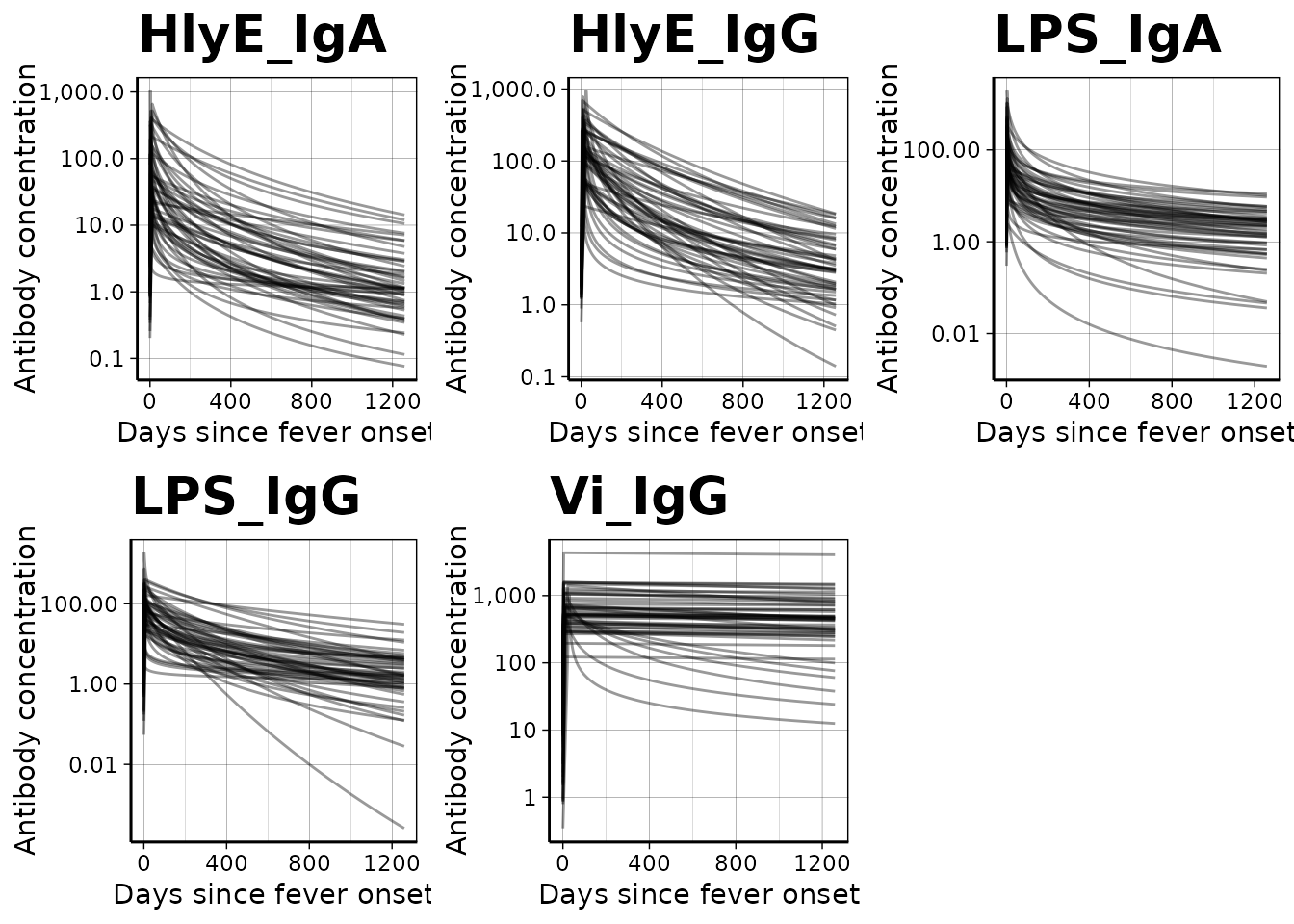
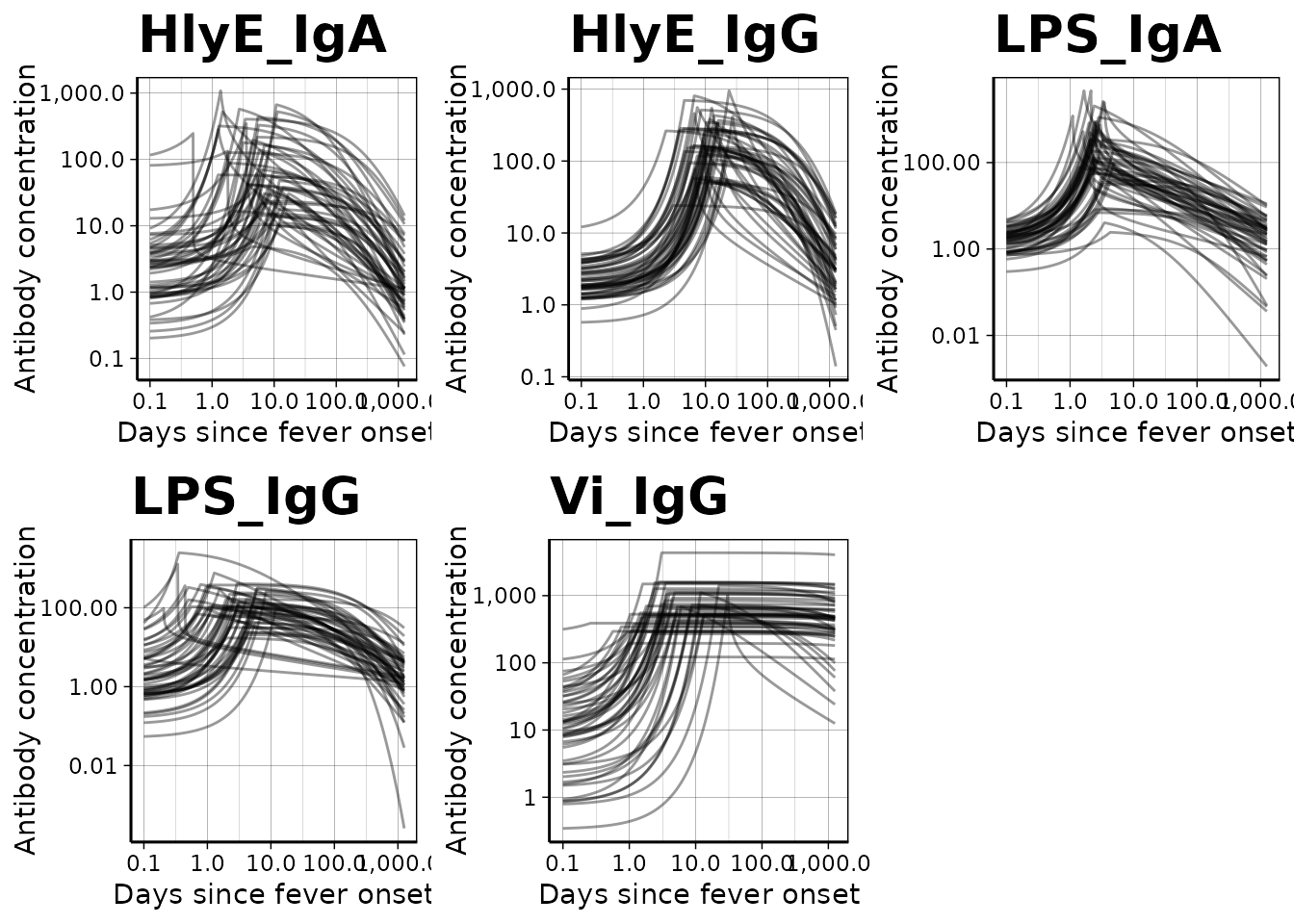
We can use a logarithmic scale for the x-axis if desired:

dmcmc %>% autoplot(log_x = TRUE, n_curves = 50)

We can graph the median, 10%, and 90% quantiles of the model using the graph.curve.params() function:

# Specify the antibody-isotype responses to include in analyses
antibodies <- c("HlyE_IgA", "HlyE_IgG")

dmcmc %>%
  graph.curve.params(antigen_isos = antibodies) %>%
  print()
#> Warning: Removed 47 rows containing missing values or values outside the scale range
#> (`geom_line()`).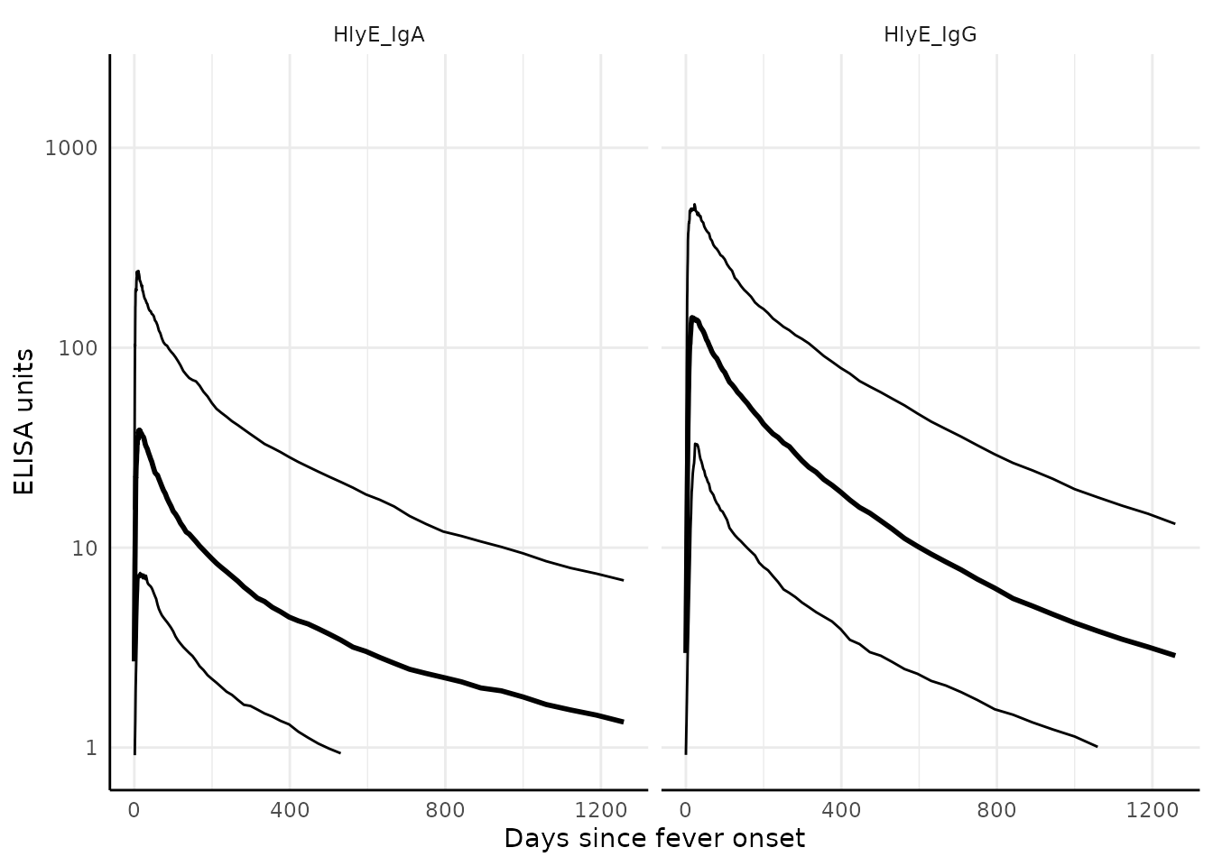

Simulate cross-sectional data

# set seed to reproduce results
set.seed(54321)

# simulated incidence rate per person-year
lambda <- 0.2
# range covered in simulations
lifespan <- c(0, 10)
# cross-sectional sample size
nrep <- 100

# biologic noise distribution
dlims <- rbind(
  "HlyE_IgA" = c(min = 0, max = 0.5),
  "HlyE_IgG" = c(min = 0, max = 0.5)
)

# generate cross-sectional data
csdata <- sim.cs(
  curve_params = dmcmc,
  lambda = lambda,
  n.smpl = nrep,
  age.rng = lifespan,
  antigen_isos = antibodies,
  n.mc = 0,
  renew.params = TRUE,
  add.noise = TRUE,
  noise_limits = dlims,
  format = "long"
)

Noise parameters

We need to provide noise parameters for the analysis; here, we define them directly in our code:

library(tibble)
cond <- tibble(
  antigen_iso = c("HlyE_IgG", "HlyE_IgA"),
  nu = c(0.5, 0.5), # Biologic noise (nu)
  eps = c(0, 0), # M noise (eps)
  y.low = c(1, 1), # low cutoff (llod)
  y.high = c(5e6, 5e6)
) # high cutoff (y.high)

Visualize data

We can plot the distribution of the antibody responses in the simulated data.

ggplot(csdata, aes(
  x = as.factor(antigen_iso),
  y = value
)) +
  geom_beeswarm(
    size = .2,
    alpha = .3,
    aes(color = antigen_iso),
    show.legend = FALSE
  ) +
  geom_boxplot(outlier.colour = NA, fill = NA) +
  scale_y_log10() +
  theme_linedraw() +
  labs(x = "antigen - isotype")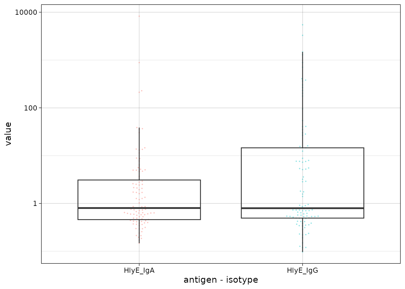

calculate log-likelihood

We can calculate the log-likelihood of the data as a function of the incidence rate directly:

ll_a <-
  log_likelihood(
    pop_data = csdata,
    curve_params = dmcmc,
    noise_params = cond,
    antigen_isos = "HlyE_IgA",
    lambda = 0.1
  ) %>%
  print()
#> [1] -240.1535

ll_g <-
  log_likelihood(
    pop_data = csdata,
    curve_params = dmcmc,
    noise_params = cond,
    antigen_isos = "HlyE_IgG",
    lambda = 0.1
  ) %>%
  print()
#> [1] -339.8803

ll_ag <-
  log_likelihood(
    pop_data = csdata,
    curve_params = dmcmc,
    noise_params = cond,
    antigen_isos = c("HlyE_IgG", "HlyE_IgA"),
    lambda = 0.1
  ) %>%
  print()
#> [1] -580.0338

print(ll_a + ll_g)
#> [1] -580.0338

graph log-likelihood

We can also graph the log-likelihoods, even without finding the MLEs, using graph_loglik():

lik_HlyE_IgA <-
  graph_loglik(
    pop_data = csdata,
    curve_params = dmcmc,
    noise_params = cond,
    antigen_isos = "HlyE_IgA",
    log_x = TRUE
  )

lik_HlyE_IgG <- graph_loglik(
  previous_plot = lik_HlyE_IgA,
  pop_data = csdata,
  curve_params = dmcmc,
  noise_params = cond,
  antigen_isos = "HlyE_IgG",
  log_x = TRUE
)

lik_both <- graph_loglik(
  previous_plot = lik_HlyE_IgG,
  pop_data = csdata,
  curve_params = dmcmc,
  noise_params = cond,
  antigen_isos = c("HlyE_IgG", "HlyE_IgA"),
  log_x = TRUE
)

print(lik_both)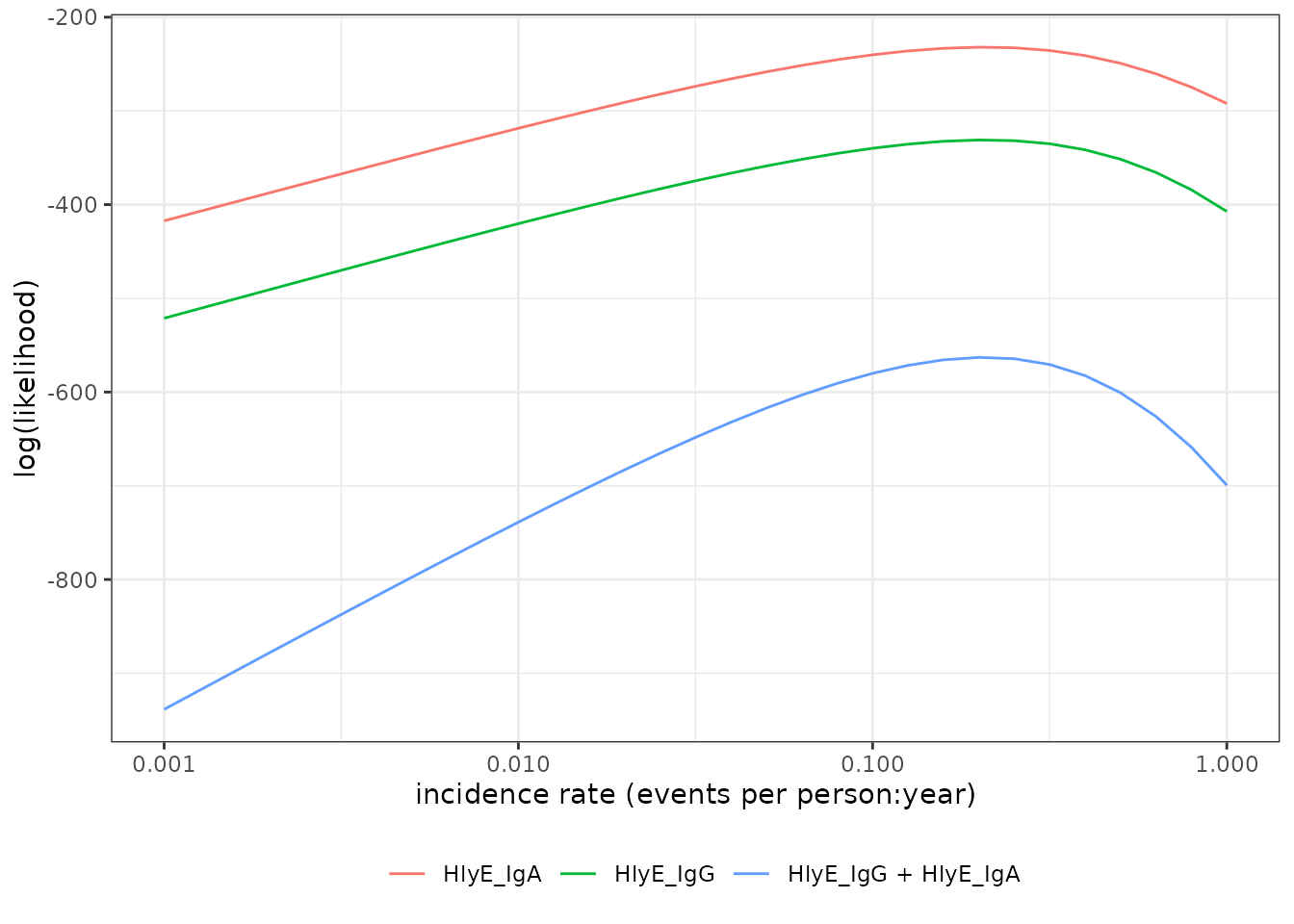

estimate incidence

We can estimate incidence with est.incidence():

est1 <- est.incidence(
  pop_data = csdata,
  curve_params = dmcmc,
  noise_params = cond,
  lambda_start = .1,
  build_graph = TRUE,
  verbose = TRUE, # print updates as the function runs
  print_graph = FALSE, # display the log-likelihood curve while
  #`est.incidence()` is running
  antigen_isos = antibodies
)
#> nrow(curve_params) = 998
#> Initial negative log-likelihood: 580.033839865286
#> building likelihood graph
#> about to call `nlm()`
#> iteration = 0
#> Step:
#> [1] 0
#> Parameter:
#> [1] -2.302585
#> Function Value
#> [1] 580.0338
#> Gradient:
#> [1] -43.94475
#> 
#> iteration = 1
#> Step:
#> [1] 0.4684939
#> Parameter:
#> [1] -1.834091
#> Function Value
#> [1] 565.4921
#> Gradient:
#> [1] -18.4184
#> 
#> iteration = 2
#> Step:
#> [1] 0.3380391
#> Parameter:
#> [1] -1.496052
#> Function Value
#> [1] 563.1786
#> Gradient:
#> [1] 6.088605
#> 
#> iteration = 3
#> Step:
#> [1] -0.08398361
#> Parameter:
#> [1] -1.580036
#> Function Value
#> [1] 562.9676
#> Gradient:
#> [1] -0.665958
#> 
#> iteration = 4
#> Step:
#> [1] 0.008280263
#> Parameter:
#> [1] -1.571755
#> Function Value
#> [1] 562.9636
#> Gradient:
#> [1] -0.9964423
#> 
#> iteration = 5
#> Step:
#> [1] 0.002099482
#> Parameter:
#> [1] -1.569656
#> Function Value
#> [1] 562.9634
#> Gradient:
#> [1] 1.11877
#> 
#> iteration = 6
#> Step:
#> [1] -1.66162e-05
#> Parameter:
#> [1] -1.569673
#> Function Value
#> [1] 562.9634
#> Gradient:
#> [1] 0.1425471
#> 
#> iteration = 7
#> Parameter:
#> [1] -1.569673
#> Function Value
#> [1] 562.9634
#> Gradient:
#> [1] -0.008628721
#> 
#> Last global step failed to locate a point lower than x.
#> Either x is an approximate local minimum of the function,
#> the function is too non-linear for this algorithm,
#> or steptol is too large.
#> Warning in est.incidence(pop_data = csdata, curve_params = dmcmc, noise_params = cond, : `nlm()` may not have reached the maximum likelihood estimate.
#> `nlm()` completed with the following convergence code:
#> 3: Last global step failed to locate a point lower than x. Either x is an approximate local minimum of the function, the function is too non-linear for this algorithm, or `stepmin` in `est.incidence()` (a.k.a. `steptol` in `nlm()`) is too large.
#> 
#> Elapsed time:
#>    user  system elapsed 
#>   0.435   0.000   0.435

We can extract summary statistics with summary():

summary(est1)
#> # A tibble: 1 × 10
#>   est.start incidence.rate     SE CI.lwr CI.upr coverage log.lik iterations
#>       <dbl>          <dbl>  <dbl>  <dbl>  <dbl>    <dbl>   <dbl>      <int>
#> 1       0.1          0.208 0.0137  0.183  0.237     0.95   -563.          7
#> # ℹ 2 more variables: antigen.isos <chr>, nlm.convergence.code <ord>

We can plot the log-likelihood curve with autoplot():

autoplot(est1)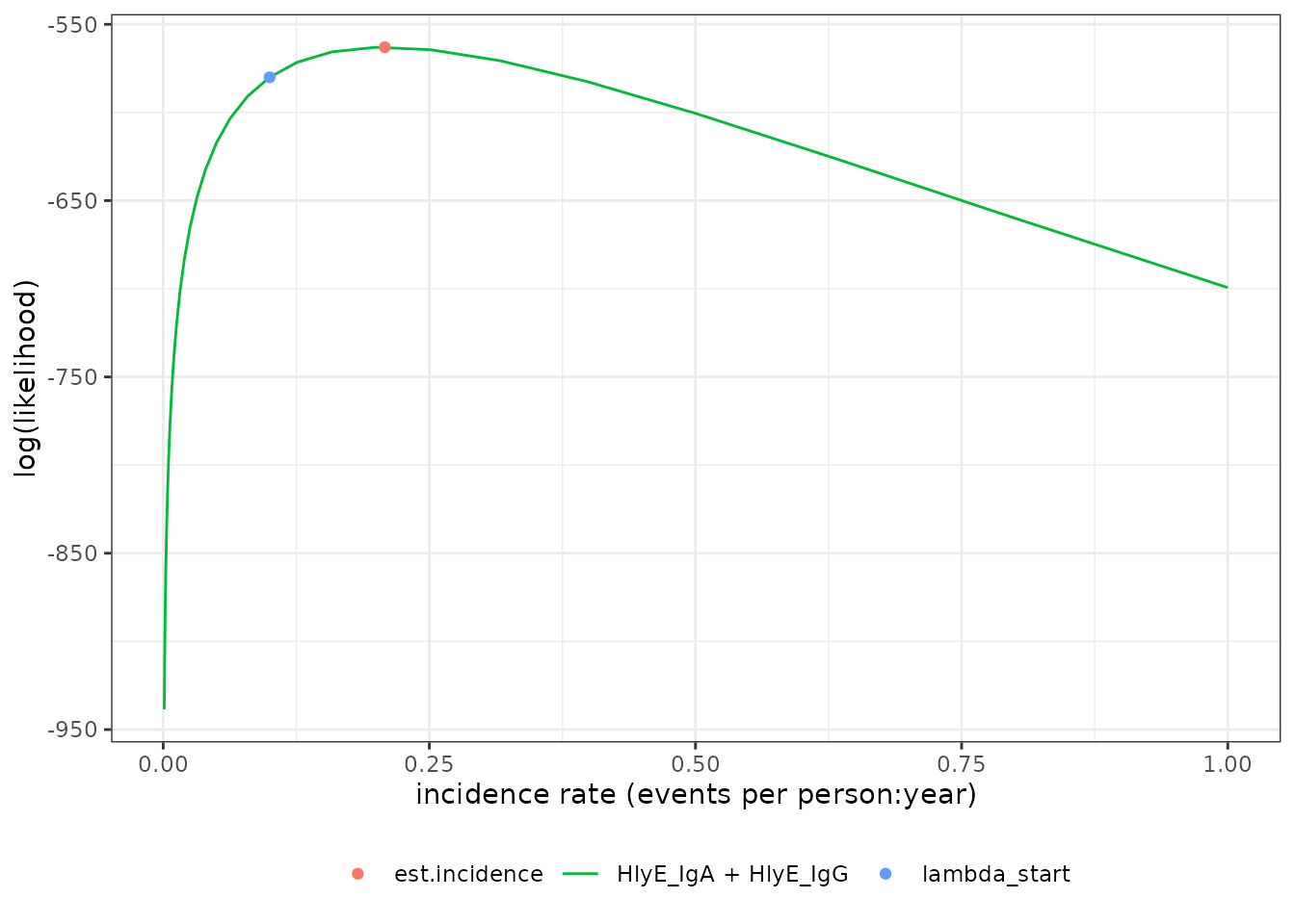

We can set the x-axis to a logarithmic scale:

autoplot(est1, log_x = TRUE)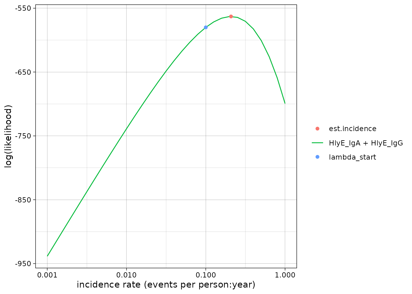

Simulate multiple clusters with different lambdas

library(parallel)
n_cores <- max(1, parallel::detectCores() - 1)
print(n_cores)
#> [1] 3

In the preceding code chunk, we have determined that we can use 3 CPU cores to run computations in parallel.

# number of clusters
nclus <- 10
# cross-sectional sample size
nrep <- 100

# incidence rate in e
lambdas <- c(.05, .1, .15, .2)

sim_df <-
  sim.cs.multi(
    n_cores = n_cores,
    lambdas = lambdas,
    nclus = nclus,
    n.smpl = nrep,
    age.rng = lifespan,
    antigen_isos = antibodies,
    renew.params = TRUE,
    add.noise = TRUE,
    curve_params = dmcmc,
    noise_limits = dlims,
    format = "long"
  )

print(sim_df)
#> # A tibble: 8,000 × 6
#>      age id    antigen_iso value lambda.sim cluster
#>    <dbl> <chr> <chr>       <dbl>      <dbl>   <int>
#>  1  3.53 1     HlyE_IgA    0.875       0.05       1
#>  2  3.53 1     HlyE_IgG    0.612       0.05       1
#>  3  2.27 2     HlyE_IgA    0.599       0.05       1
#>  4  2.27 2     HlyE_IgG    0.481       0.05       1
#>  5  9.05 3     HlyE_IgA    0.577       0.05       1
#>  6  9.05 3     HlyE_IgG    0.440       0.05       1
#>  7  5.94 4     HlyE_IgA    0.873       0.05       1
#>  8  5.94 4     HlyE_IgG    0.866       0.05       1
#>  9  9.88 5     HlyE_IgA    0.633       0.05       1
#> 10  9.88 5     HlyE_IgG    0.152       0.05       1
#> # ℹ 7,990 more rows

We can plot the distributions of the simulated responses:

sim_df %>% ggplot() +
  aes(
    x = as.factor(cluster),
    y = value
  ) +
  geom_beeswarm(size = .2, alpha = .3, aes(color = antigen_iso)) +
  geom_boxplot(outlier.colour = NA, fill = NA) +
  scale_y_log10() +
  facet_wrap(~ antigen_iso + lambda.sim, nrow = 2) +
  theme_linedraw()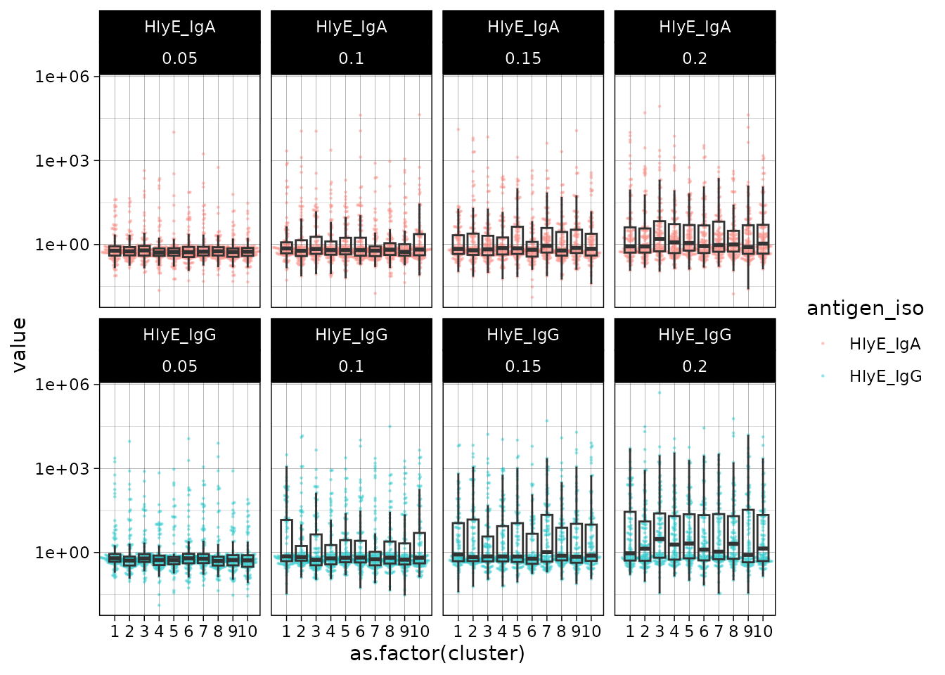

Estimate incidence in each cluster

ests <-
  est.incidence.by(
    pop_data = sim_df,
    curve_params = dmcmc,
    noise_params = cond,
    num_cores = n_cores,
    strata = c("lambda.sim", "cluster"),
    curve_strata_varnames = NULL,
    noise_strata_varnames = NULL,
    verbose = TRUE,
    build_graph = TRUE, # slows down the function substantially
    antigen_isos = c("HlyE_IgG", "HlyE_IgA")
  )
#> Data has been stratified.
#> Here are the strata that will be analyzed:
#> # A tibble: 40 × 4
#>    Stratum    lambda.sim cluster     n
#>    <chr>           <dbl>   <int> <int>
#>  1 Stratum 1        0.05       1   100
#>  2 Stratum 2        0.05       2   100
#>  3 Stratum 3        0.05       3   100
#>  4 Stratum 4        0.05       4   100
#>  5 Stratum 5        0.05       5   100
#>  6 Stratum 6        0.05       6   100
#>  7 Stratum 7        0.05       7   100
#>  8 Stratum 8        0.05       8   100
#>  9 Stratum 9        0.05       9   100
#> 10 Stratum 10       0.05      10   100
#> # ℹ 30 more rows
#> Setting up parallel processing with `num_cores` = 3.
#> Elapsed time for parallelized code:
#>    user  system elapsed 
#>   0.146   0.026  17.340

summary(ests) produces a tibble() with some extra meta-data:

summary(ests)
#> Warning in FUN(X[[i]], ...): `nlm()` produced a negative hessian; something is wrong with the numerical derivatives.
#> The standard error of the incidence rate estimate cannot be calculated.
#> Warning in sqrt(var.log.lambda): NaNs produced
#> Warning in FUN(X[[i]], ...): `nlm()` produced a negative hessian; something is wrong with the numerical derivatives.
#> The standard error of the incidence rate estimate cannot be calculated.
#> Warning in sqrt(var.log.lambda): NaNs produced
#> Warning in FUN(X[[i]], ...): `nlm()` produced a negative hessian; something is wrong with the numerical derivatives.
#> The standard error of the incidence rate estimate cannot be calculated.
#> Warning in sqrt(var.log.lambda): NaNs produced
#> Warning in FUN(X[[i]], ...): `nlm()` produced a negative hessian; something is wrong with the numerical derivatives.
#> The standard error of the incidence rate estimate cannot be calculated.
#> Warning in sqrt(var.log.lambda): NaNs produced
#> Warning in FUN(X[[i]], ...): `nlm()` produced a negative hessian; something is wrong with the numerical derivatives.
#> The standard error of the incidence rate estimate cannot be calculated.
#> Warning in sqrt(var.log.lambda): NaNs produced
#> Seroincidence estimated given the following setup:
#> a) Antigen isotypes   : HlyE_IgG, HlyE_IgA 
#> b) Strata       : lambda.sim, cluster 
#> 
#>  Seroincidence estimates:
#> # A tibble: 40 × 14
#>    Stratum    lambda.sim cluster     n est.start incidence.rate      SE CI.lwr
#>    <chr>           <dbl>   <int> <int>     <dbl>          <dbl>   <dbl>  <dbl>
#>  1 Stratum 1        0.05       1   100       0.1         0.0680 0.0108  0.0498
#>  2 Stratum 2        0.05       2   100       0.1         0.0603 0.00949 0.0443
#>  3 Stratum 3        0.05       3   100       0.1         0.0556 0.00925 0.0401
#>  4 Stratum 4        0.05       4   100       0.1         0.0568 0.00972 0.0406
#>  5 Stratum 5        0.05       5   100       0.1         0.0350 0.00719 0.0234
#>  6 Stratum 6        0.05       6   100       0.1         0.0558 0.00915 0.0405
#>  7 Stratum 7        0.05       7   100       0.1         0.0687 0.0109  0.0503
#>  8 Stratum 8        0.05       8   100       0.1         0.0404 0.00787 0.0276
#>  9 Stratum 9        0.05       9   100       0.1         0.0458 0.00826 0.0322
#> 10 Stratum 10       0.05      10   100       0.1         0.0423 0.00791 0.0293
#> # ℹ 30 more rows
#> # ℹ 6 more variables: CI.upr <dbl>, coverage <dbl>, log.lik <dbl>,
#> #   iterations <int>, antigen.isos <chr>, nlm.convergence.code <ord>

We can explore the summary table interactively using DT::datatable()

library(DT)
summary(ests) %>%
  DT::datatable() %>%
  DT::formatRound(
    columns = c(
      "incidence.rate",
      "SE",
      "CI.lwr",
      "CI.upr",
      "log.lik"
    )
  )
#> Warning in FUN(X[[i]], ...): `nlm()` produced a negative hessian; something is wrong with the numerical derivatives.
#> The standard error of the incidence rate estimate cannot be calculated.
#> Warning in sqrt(var.log.lambda): NaNs produced
#> Warning in FUN(X[[i]], ...): `nlm()` produced a negative hessian; something is wrong with the numerical derivatives.
#> The standard error of the incidence rate estimate cannot be calculated.
#> Warning in sqrt(var.log.lambda): NaNs produced
#> Warning in FUN(X[[i]], ...): `nlm()` produced a negative hessian; something is wrong with the numerical derivatives.
#> The standard error of the incidence rate estimate cannot be calculated.
#> Warning in sqrt(var.log.lambda): NaNs produced
#> Warning in FUN(X[[i]], ...): `nlm()` produced a negative hessian; something is wrong with the numerical derivatives.
#> The standard error of the incidence rate estimate cannot be calculated.
#> Warning in sqrt(var.log.lambda): NaNs produced
#> Warning in FUN(X[[i]], ...): `nlm()` produced a negative hessian; something is wrong with the numerical derivatives.
#> The standard error of the incidence rate estimate cannot be calculated.
#> Warning in sqrt(var.log.lambda): NaNs produced

We can plot the likelihood for a single simulated cluster by subsetting that simulation in ests and calling plot():

autoplot(ests[1])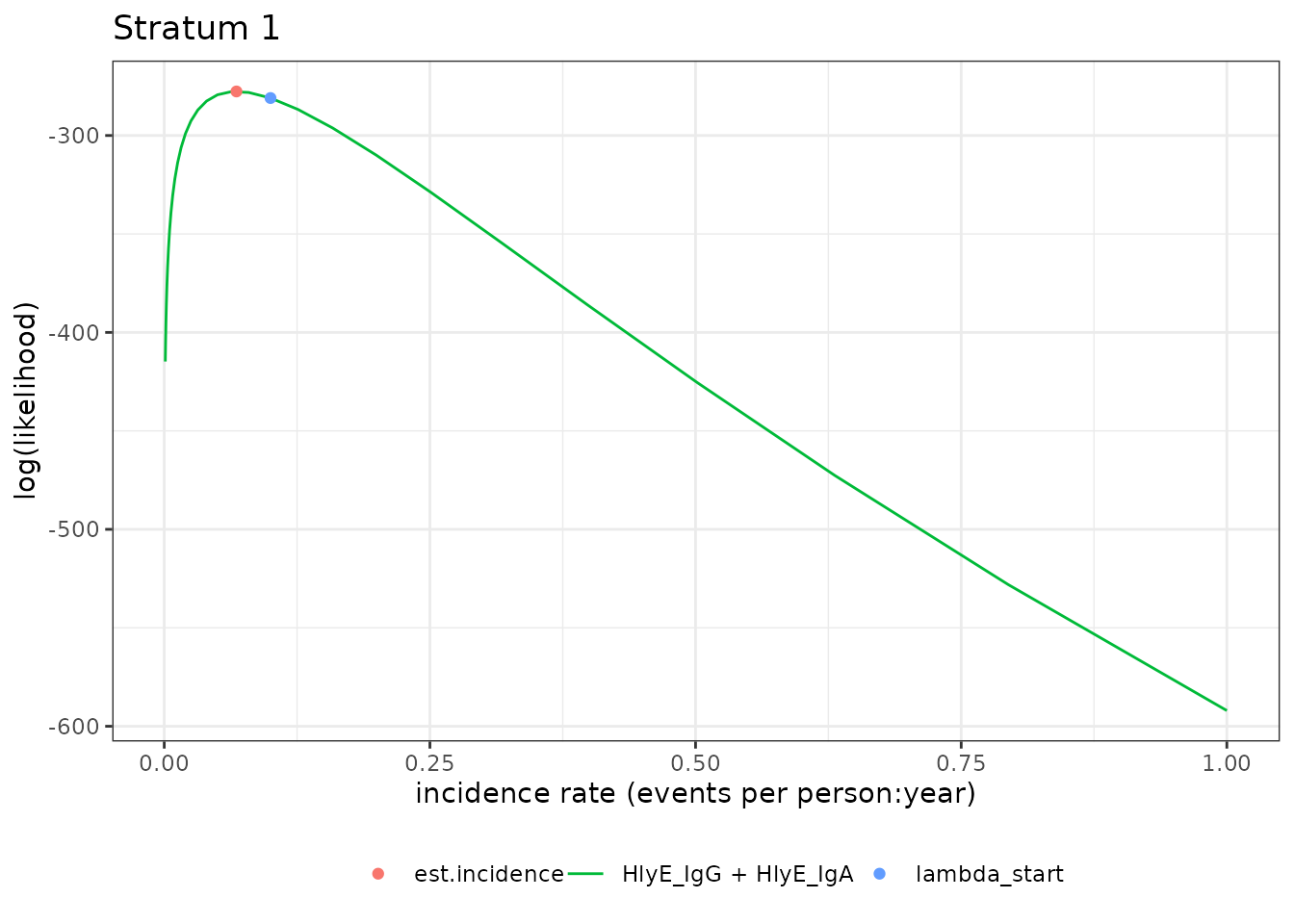

We can also plot log-likelihood curves for several clusters at once (your computer might struggle to plot many at once):

autoplot(ests[1:5])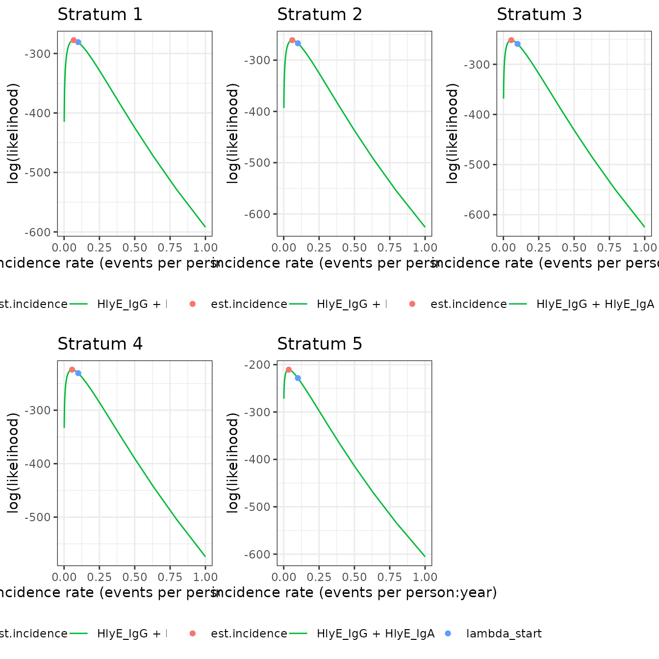

The log_x argument also works here:

autoplot(ests[1:5], log_x = TRUE)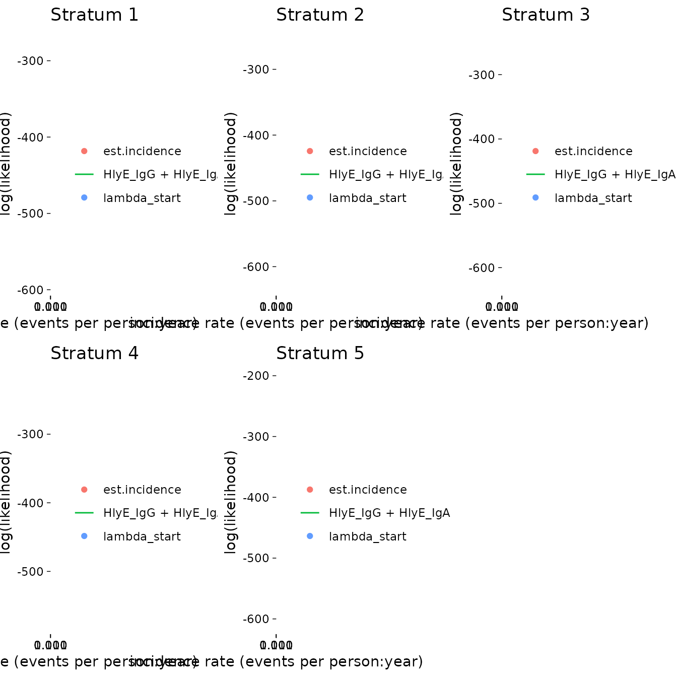

nlm() convergence codes

Make sure to check the nlm() exit codes (codes 3-5 indicate possible non-convergence):

summary(ests) %>%
  as_tibble() %>% # removes extra meta-data
  select(Stratum, nlm.convergence.code) %>%
  filter(nlm.convergence.code > 2)
#> Warning in FUN(X[[i]], ...): `nlm()` produced a negative hessian; something is wrong with the numerical derivatives.
#> The standard error of the incidence rate estimate cannot be calculated.
#> Warning in sqrt(var.log.lambda): NaNs produced
#> Warning in FUN(X[[i]], ...): `nlm()` produced a negative hessian; something is wrong with the numerical derivatives.
#> The standard error of the incidence rate estimate cannot be calculated.
#> Warning in sqrt(var.log.lambda): NaNs produced
#> Warning in FUN(X[[i]], ...): `nlm()` produced a negative hessian; something is wrong with the numerical derivatives.
#> The standard error of the incidence rate estimate cannot be calculated.
#> Warning in sqrt(var.log.lambda): NaNs produced
#> Warning in FUN(X[[i]], ...): `nlm()` produced a negative hessian; something is wrong with the numerical derivatives.
#> The standard error of the incidence rate estimate cannot be calculated.
#> Warning in sqrt(var.log.lambda): NaNs produced
#> Warning in FUN(X[[i]], ...): `nlm()` produced a negative hessian; something is wrong with the numerical derivatives.
#> The standard error of the incidence rate estimate cannot be calculated.
#> Warning in sqrt(var.log.lambda): NaNs produced
#> # A tibble: 8 × 2
#>   Stratum    nlm.convergence.code
#>   <chr>      <ord>               
#> 1 Stratum 12 3                   
#> 2 Stratum 13 3                   
#> 3 Stratum 21 3                   
#> 4 Stratum 29 3                   
#> 5 Stratum 31 3                   
#> 6 Stratum 34 3                   
#> 7 Stratum 36 3                   
#> 8 Stratum 39 3

Solutions to nlm() exit codes 3-5:

• 3: decrease the stepmin argument to est.incidence()/est.incidence.by()
• 4: increase the iterlim argument to est.incidence()/est.incidence.by()
• 5: increase the stepmax argument to est.incidence()/est.incidence.by()

We can extract the indices of problematic strata, if there are any:

problem_strata <-
  which(summary(ests)$nlm.convergence.code > 2) %>%
  print()
#> Warning in FUN(X[[i]], ...): `nlm()` produced a negative hessian; something is wrong with the numerical derivatives.
#> The standard error of the incidence rate estimate cannot be calculated.
#> Warning in sqrt(var.log.lambda): NaNs produced
#> Warning in FUN(X[[i]], ...): `nlm()` produced a negative hessian; something is wrong with the numerical derivatives.
#> The standard error of the incidence rate estimate cannot be calculated.
#> Warning in sqrt(var.log.lambda): NaNs produced
#> Warning in FUN(X[[i]], ...): `nlm()` produced a negative hessian; something is wrong with the numerical derivatives.
#> The standard error of the incidence rate estimate cannot be calculated.
#> Warning in sqrt(var.log.lambda): NaNs produced
#> Warning in FUN(X[[i]], ...): `nlm()` produced a negative hessian; something is wrong with the numerical derivatives.
#> The standard error of the incidence rate estimate cannot be calculated.
#> Warning in sqrt(var.log.lambda): NaNs produced
#> Warning in FUN(X[[i]], ...): `nlm()` produced a negative hessian; something is wrong with the numerical derivatives.
#> The standard error of the incidence rate estimate cannot be calculated.
#> Warning in sqrt(var.log.lambda): NaNs produced
#> [1] 12 13 21 29 31 34 36 39

If any clusters had problems, we can take a look:

if (length(problem_strata) > 0) {
  autoplot(ests[problem_strata], log_x = TRUE)
}

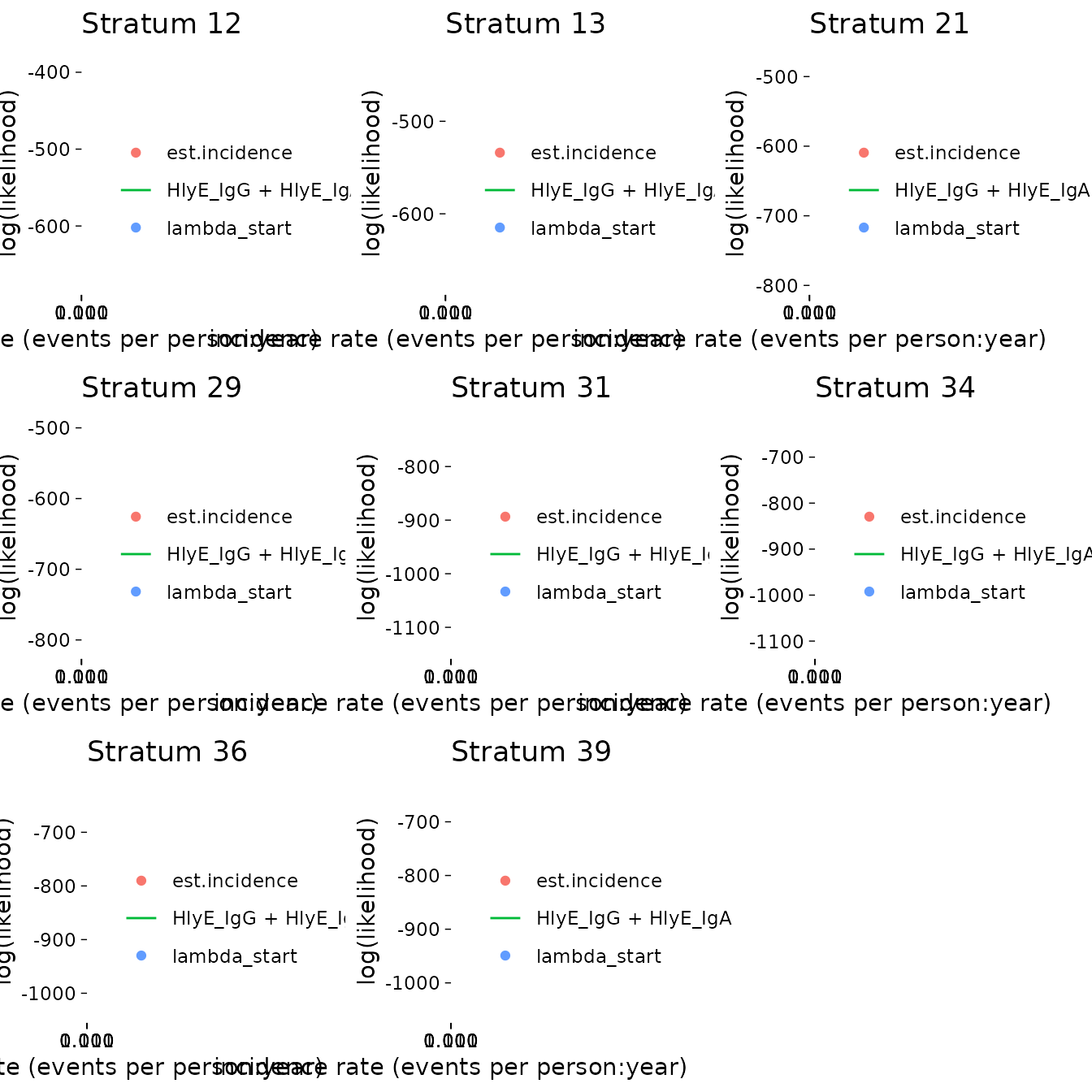
If any of the fits don’t appear to be at the maximum likelihood, we should re-run those clusters, adjusting the nlm() settings appropriately, to be sure.

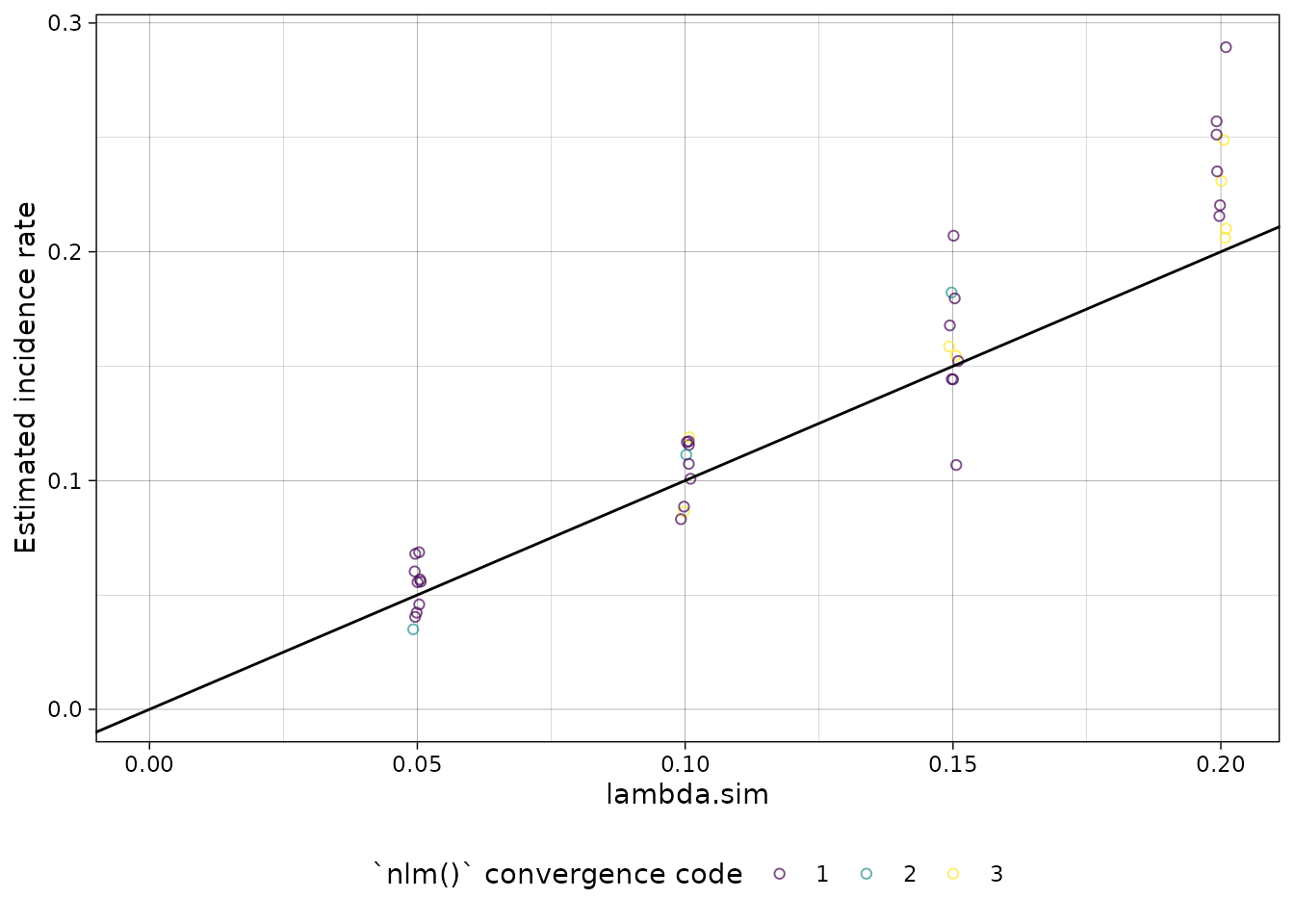
plot distribution of estimates by simulated incidence rate

Finally, we can look at our simulation results:

library(ggplot2)
summary(ests) %>%
  autoplot(xvar = "lambda.sim") +
  ggplot2::geom_abline(
    ggplot2::aes(intercept = 0, slope = 1)
  )
#> Warning in FUN(X[[i]], ...): `nlm()` produced a negative hessian; something is wrong with the numerical derivatives.
#> The standard error of the incidence rate estimate cannot be calculated.
#> Warning in sqrt(var.log.lambda): NaNs produced
#> Warning in FUN(X[[i]], ...): `nlm()` produced a negative hessian; something is wrong with the numerical derivatives.
#> The standard error of the incidence rate estimate cannot be calculated.
#> Warning in sqrt(var.log.lambda): NaNs produced
#> Warning in FUN(X[[i]], ...): `nlm()` produced a negative hessian; something is wrong with the numerical derivatives.
#> The standard error of the incidence rate estimate cannot be calculated.
#> Warning in sqrt(var.log.lambda): NaNs produced
#> Warning in FUN(X[[i]], ...): `nlm()` produced a negative hessian; something is wrong with the numerical derivatives.
#> The standard error of the incidence rate estimate cannot be calculated.
#> Warning in sqrt(var.log.lambda): NaNs produced
#> Warning in FUN(X[[i]], ...): `nlm()` produced a negative hessian; something is wrong with the numerical derivatives.
#> The standard error of the incidence rate estimate cannot be calculated.
#> Warning in sqrt(var.log.lambda): NaNs produced