Introduction to seroincidence estimation

Overview

Defining incidence

The incidence rate of a disease over a specific time period is the rate at which individuals in a population are acquiring the disease during that time period [@Noordzij2010diseasemeasures].

Example: if there are 10 new cases of typhoid in a population of 1000 persons during a one month time period, then the incidence rate for that time period is 10 new cases per 1000 persons per month.

Mathematical definition of incidence

More mathematically, the incidence rate at a given time point is the derivative (i.e., the current rate of change over time) of the expected cumulative count of infections per person at risk, at that time:

$$\frac{d}{dt} \mathbb{E}\left[\frac{C(t)}{n} \mid N(t) =n\right]$$

where $C(t)$ is the cumulative total number of infections in the population of interest, and $N(t)$ is the number of individuals at risk at time $t$.

Scale of incidence rates

In both definitions, the units for an incidence rate are “# new infections per # persons at risk per time duration”; for example, “new infections per 1000 persons per year”.

For convenience, we can rescale the incidence rate to make it easier to understand; for example, we might express incidence as “# new infections per 1000 persons per year” or “# new infections per 100,000 persons per day”, etc.

Incidence from an individual’s perspective

From the perspective of an individual in the population:

• the incidence rate (at a given time point ($t$) is the instantaneous probability (density) of becoming infected at that time point, given that they are at risk at that time point.

• That is, the incidence rate is a hazard rate.

• Notation: let’s use $\lambda_{t}$ to denote the incidence rate at time $t$.

Estimating incidence from cross-sectional antibody surveys

Cross-sectional antibody surveys

Typically, it is difficult to estimate changes from a single time point. However, we can sometimes make assumptions that allow us to do so. In particular, if we assume that the incidence rate is constant over time, then we can estimate incidence from a single cross-sectional survey.

We will need two pieces of notation to formalize this process.

• We recruit participants from the population of interest.

• For each survey participant, we measure antibody levels $(Y)$ for the disease of interest

• Each participant was most recently infected at some time $(T)$prior to when we measured their antibodies.

• If a participant has never been infected since birth, then $T$ is undefined.

• $T$ is a latent, unobserved variable.

• We don’t directly observe $T$; we only observe $Y$, which we hope tells us something about $T$ and $\lambda$.

Modeling assumptions

We assume that:

• The incidence rate is approximately constant over time and across the population (“constant and homogenous incidence”)

• that is: $$\lambda_{i,t} = \lambda, \forall i,t$$

(We can analyze subpopulations separately to make homogeneity more plausible.)

• Participants are always at risk of a new infection, regardless of how recently they have been infected (“no lasting immunity”).

(For diseases like typhoid, the no-immunity assumption may not hold exactly, but hopefully approximately; modeling the effects of re-exposure during an active infection is on our to-do list).

Time since infection and incidence

Under those assumptions:

• $T$ has an exponential distribution:

$$\mathbb{p}(T=t) = \lambda \exp{\left\{-\lambda t\right\}}$$

• More precisely, the distribution is exponential truncated by age at observation ($a$):

$$\mathbb{p}(T=t|A=a) = 1_{t \in[0,a]}\lambda \exp{\left\{-\lambda t\right\}} + 1_{t = \text{NA}} \exp{\left\{-\lambda a\right\}}$$

• the rate parameter $\lambda$ is the incidence rate

This is a time-to-event model, looking backwards in time from the survey date (when the blood sample was collected).

The probability that an individual was last infected $t$ days ago, $p(T=t)$, is equal to the probability of being infected at time $t$ (i.e., the incidence rate at time $t$, $\lambda$) times the probability of not being infected after time $t$, which turns out to be $\exp(-\lambda t)$.

The distribution of $T$ is truncated by the patient’s birth date; the probability that they have never been infected is $\exp{\left\{-\lambda a\right\}}$, where $a$ is the patient’s age at the time of the survey.

Likelihood of latent infection times

If we could observe $T$, then we could estimate $\lambda$ using a typical maximum likelihood approach.

Starting with the likelihood: Taking the logarithm of the likelihood: Taking the derivative of that log-likelihood to find the score function: Setting the score function equal to 0 to find the score equation, and solving the score equation for $\lambda$ to find the maximum likelihood estimate:

• $$\mathcal{L}^*(\lambda) = \prod_{i=1}^n \mathbb{p}(T=t_i) = \prod_{i=1}^n \lambda \exp(-\lambda t_i)$$

• $$\ell^*(\lambda) = \log{\left\{\mathcal{L}^*(\lambda)\right\}} = \sum_{i=1}^n \log{\left\{\lambda\right\}} -\lambda t_i$$

• $$\ell^{*'}(\lambda) = \sum_{i=1}^n \lambda^{-1} - t_i$$

• $$\hat{\lambda}_{\text{ML}} = \frac{n}{\sum_{i=1}^n t_i} = \frac{1}{\bar{t}}$$

The MLE turns out to be the inverse of the mean.

Example log-likelihood curves

Here’s what that would look like:

library(serocalculator)
library(dplyr)

Attaching package: 'dplyr'

The following objects are masked from 'package:stats':

    filter, lag

The following objects are masked from 'package:base':

    intersect, setdiff, setequal, union

# Import longitudinal antibody parameters from OSF
curves <-
  "https://osf.io/download/rtw5k/" %>%
  load_curve_params() %>%
  filter(iter < 50)

# Import cross-sectional data from OSF and rename required variables:
xs_data <-
  "https://osf.io/download//n6cp3/" %>%
  load_pop_data()

noise <- url("https://osf.io/download//hqy4v/") %>% readRDS()

lik_HlyE_IgA <- graph_loglik(
  pop_data = xs_data,
  curve_params = curves,
  noise_params = noise,
  antigen_isos = "HlyE_IgA",
  log_x = TRUE
)

lik_HlyE_IgG <- graph_loglik(
  previous_plot = lik_HlyE_IgA,
  pop_data = xs_data,
  curve_params = curves,
  noise_params = noise,
  antigen_isos = "HlyE_IgG",
  log_x = TRUE
)

lik_both <- graph_loglik(
  previous_plot = lik_HlyE_IgG,
  pop_data = xs_data,
  curve_params = curves,
  noise_params = noise,
  antigen_isos = c("HlyE_IgG", "HlyE_IgA"),
  log_x = TRUE
)

print(lik_both)

Figure 1: Example log(likelihood) curves

standard error

The standard error of the estimate is approximately equal to the inverse of the rate of curvature (2nd derivative, aka Hessian) in the log-likelihood function, at the maximum:

more curvature -> likelihood peak is clearer -> smaller standard errors

Likelihood of observed data

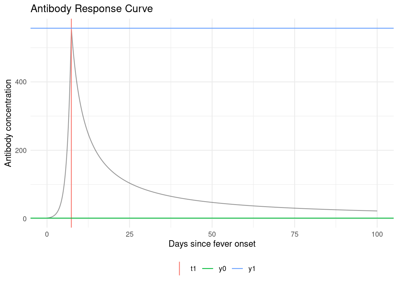
Unfortunately, we don’t observe infection times $T$; we only observe antibody levels ${Y}$. So things get a little more complicated.

In short, we are hoping that we can estimate $T$ (time since last infection) from $Y$ (current antibody levels). If we could do that, then we could plug in our estimates $\hat t_i$ into that likelihood above, and estimate $\lambda$ as previously.

We’re actually going to do something a little more nuanced; instead of just using one value for $\hat t$, we are going to consider all possible values of $t$ for each individual.

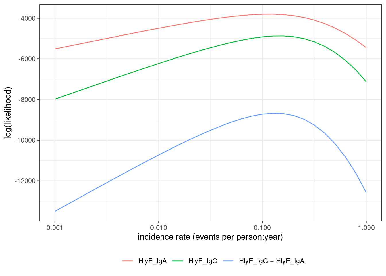
We need to link the data we actually observed to the incidence rate.

The likelihood of an individual’s observed data, $\mathbb{p}(Y=y)$, can be expressed as an integral over the joint likelihood of $Y$ and $T$ (using the Law of Total Probability):

• $$\mathbb{p}(Y=y) = \int_t \mathbb{p}(Y=y,T=t)dt$$

Further, we can express the joint probability $p(Y=y,T=t)$ as the product of $p(T=t)$ and $p(Y=y|T=t)$ the “antibody response curve after infection”. That is:

• $$\mathbb{p}(Y=y,T=t) = \mathbb{p}(Y=y|T=t) \mathbb{p}(T=t)$$

Antibody response curves

Figure 2: Antibody response curves, $p(Y=y|T=t)$, for typhoid

Putting it all together

Substituting $p(Y=y,T=t) = p(Y=y|T=t)P(T=t)$ into the previous expression for $p(Y=y)$:

$$\begin{aligned} p(Y=y) &= \int_t p(Y=y|T=t)P(T=t) dt \end{aligned}$$

Composing the likelihood

Now, the likelihood of the observed data $\mathbf{y} = (y_1, y_2, ..., y_n)$ is:

$$\begin{aligned} \mathcal{L}(\lambda) &= \prod_{i=1}^n p(Y=y_i) \\&= \prod_{i=1}^n \int_t p(Y=y_i|T=t)p_\lambda(T=t)dt\\ \end{aligned}$$

If we know $p(Y=y|T=t)$, then we can maximize $\mathcal{L}(\lambda)$ over $\lambda$ to find the “maximum likelihood estimate” (MLE) of $\lambda$, denoted $\hat\lambda$.

Finding the MLE numerically

The likelihood of $Y$ involves the product of integrals, so the log-likelihood involves the sum of the logs of integrals:

$$\begin{aligned} \log \mathcal{L} (\lambda) &= \log \prod_{i=1}^n \int_t p(Y=y_i|T=t)p_\lambda(T=t)dt\\ &= \sum_{i=1}^n \log\left\{\int_t p(Y=y_i|T=t)p_\lambda(T=t)dt\right\}\\ \end{aligned}$$

The derivative of this expression doesn’t come out cleanly, so we will use a numerical method (specifically, a Newton-type algorithm, implemented by stats::nlm()) to find the MLE and corresponding standard error.

Modeling the seroresponse kinetics curve

Now, we need a model for the antibody response to infection, $\mathbb{p}(Y=y|T=t)$. The current version of the serocalculator package uses a two-phase model for the shape of the seroresponse [@Teunis_2016].

Model for active infection period

The first phase of the model represents the active infection period, and uses a simplified Lotka-Volterra predator-prey model [@volterra1928variations] where the pathogen is the prey and the antibodies are the predator:

Notation:

• $x(t)$: Pathogen concentration at time $t$
• $y(t)$: Antibody concentration at time $t$

Model:

• $$x'(t) = \alpha x(t) - \beta y(t)$$
• $$y'(t) = \delta y(t)$$

With baseline antibody concentration $y(0) = y_{0}$ and initial pathogen concentration $x(0) = x_{0}$.

Compared to the standard LV model:

• the predation term with the $\beta$ coefficient is missing the prey concentration $x(t)$ factor; we assume that the efficiency of predation doesn’t depend on pathogen concentration.

• the differential equation for predator density is missing the predator death rate term $-\gamma y(t)$; we assume that as long as there are any pathogens present, the antibody decay rate is negligible compared to the growth rate.

• the predator growth rate term $\delta y(t)$ is missing the prey density factor $x(t)$ we assume that as long as there are any pathogens present, the antibody concentration grows at the same exponential rate.

These omissions were made to simplify the estimation process, under the assumption that they are negligible compared to the other terms in the model.

Model for post-infection antibody decay

• $$b(t) = 0$$

• $$y^{\prime}(t) = -\alpha y(t)^r$$

Antibody decay is different from exponential (log–linear) decay. When the shape parameter $r > 1$, log concentrations decrease rapidly after infection has terminated, but decay then slows down and low antibody concentrations are maintained for a long period. If $r = 1$, this model reduces to exponential decay with decay rate $\alpha$.

Putting it all together

The serum antibody response $y(t)$ can be written as

$$y(t) = y_{+}(t) + y_{-}(t)$$

where

$$\begin{align} y_{+}(t) & = y_{0}\text{e}^{\mu t}[0\leq t <t_{1}]\\ y_{-}(t) & = y_{1}\left(1+(r-1)y_{1}^{r-1}\alpha(t-t_{1})\right)^{-\frac{1}{r-1}}[t_{1}\le t < \infty] \end{align}$$

---

Since the peak level is $y_{1} = y_{0}\text{e}^{\mu t_{1}}$ the growth rate $\mu$ can be written as $$\mu = \frac{1}{t_{1}}\log\left(\frac{y_{1}}{y_{0}}\right)$$

---

cur_ai = "HlyE_IgG"

library(serocalculator)
library(dplyr)
# Import longitudinal antibody parameters from OSF
curves <-
  "https://osf.io/download/rtw5k/" %>%
  load_curve_params() %>%
  filter(iter < 50)

curve1 =
  curves %>%
  filter(
    # iter %in% 1:10,
    iter == 5,
         antigen_iso == cur_ai)

library(ggplot2)

curve1 %>%
serocalculator:::plot_curve_params_one_ab(
  log_y = FALSE
) +
  xlim(0, 100) +
  theme_minimal() +
  geom_vline(
    aes(xintercept = curve1$t1,
        col = "t1")
  ) +

  geom_hline(
    aes(yintercept = curve1$y0,
        col = "y0")
  ) +


  geom_hline(
    aes(yintercept = curve1$y1,
        col = "y1")
  ) +
  # geom_point(
  #   data = curve1,
  #   aes(
  #     x = t1,
  #     y = y1,
  #     col = "(t1,y1)"
  #   )
  # ) +
  theme(legend.position = "bottom") +
  labs(col = "")

Scale for x is already present.
Adding another scale for x, which will replace the existing scale.

Figure 3: An example kinetics curve for HlyE IgG

The antibody level at $t=0$ is $y_{0}$; the rising branch ends at $t = t_{1}$ where the peak antibody level $y_{1}$ is reached. Any antibody level $y(t) \in (y_{0}, y_{1})$ eventually occurs twice.

---

An interactive Shiny app that allows the user to manipulate the model parameters is available at:

https://ucdserg.shinyapps.io/antibody-kinetics-model-2/

QR code for shiny app

Biological noise

When we measure antibody concentrations in a blood sample, we are essentially counting molecules (using biochemistry).

We might miss some of the antibodies (undercount, false negatives) and we also might incorrectly count some other molecules that aren’t actually the ones we are looking for (overcount, false positives, cross-reactivity).

We are more concerned about overcount (cross-reactivity) than undercount. For a given antibody, we can do some analytical work beforehand to estimate the distribution of overcounts, and add that to our model $p(Y=y|T=t)$.

Notation:

• $y_\text{obs}$: measured serum antibody concentration
• $y_\text{true}$: “true” serum antibody concentration
• $\epsilon_b$: noise due to probe cross-reactivity

Model:

• $y_\text{obs} = y_\text{true} + \epsilon_b$
• $\epsilon_b \sim \text{Unif}(0, \nu)$

$\nu$ needs to be pre-estimated using negative controls, typically using the 95th percentile of the distribution of antibody responses to the antigen-isotype in a population with no exposure.

Measurement noise

There are also some other sources of noise in our bioassays; user differences in pipetting technique, random ELISA plate effects, etc. This noise can cause both overcount and undercount. We can also estimate the magnitude of this noise source, and include it in $p(Y=y|T=t)$.

Measurement noise, $\varepsilon$ (“epsilon”), represents measurement error from the laboratory testing process. It is defined by a CV (coefficient of variation) as the ratio of the standard deviation to the mean for replicates. Note that the CV should ideally be measured across plates rather than within the same plate.

References