Scrub Typhus Seroincidence Vignette

Introduction

This vignette reproduces the analysis for: Estimating the seroincidence of scrub typhus using antibody dynamics following infection (Aiemjoy et al. (Accepted Feb 2024)).

Methods

The serocalculator R package provides a rapid and computationally simple method for calculating seroconversion rates, as originally published in Simonsen et al. (2009) and Teunis et al. (2012), and further developed in subsequent publications by deGraaf et al. (2014), Teunis et al. (2016), and Teunis and Eijkeren (2020). In short, longitudinal seroresponses from confirmed cases with a known symptom onset date are assumed to represent the time course of human serum antibodies against a specific pathogen. Therefore, by using these longitudinal antibody dynamics with any cross–sectional sample of the same antibodies in a human population, an incidence estimate can be calculated.

The Seroincidence Estimator

The serocalculator package was designed to calculate the incidence of seroconversion by using the longitudinal seroresponse characteristics. The distribution of serum antibody concentrations in a cross–sectional population sample is calculated as a function of the longitudinal seroresponse and the frequency of seroconversion (or seroincidence). Given the seroresponse, this marginal distribution of antibody concentrations can be fitted to the cross-sectional data and thereby providing a means to estimate the seroincidence.

Scrub Typhus Seroincidence

Scrub typhus, a vector-borne bacterial infection, is an important but neglected disease globally. Accurately characterizing burden is challenging due to non-specific symptoms and limited diagnostics. Prior seroepidemiology studies have struggled to find consensus cutoffs that permit comparing estimates across contexts and time. In this study, we present a novel approach that does not require a cutoff and instead uses information about antibody kinetics after infection to estimate seroincidence. We use data from three cohorts of scrub typhus patients in Chiang Rai, Thailand, and Vellore, India to characterize antibody kinetics after infection and two population serosurveys in the Kathmandu valley, Nepal, and Tamil Nadu, India to estimate seroincidence. The samples were tested for IgM and IgG responses to Orientia tsutsugamushi-derived recombinant 56-kDa antigen using commercial ELISA kits. We used Bayesian hierarchical models to characterize antibody responses after scrub typhus infection and used the joint distributions of the peak antibody titers and decay rates to estimate population-level incidence rates in the cross-sectional serosurveys.

Load packages

The first step in conducting this analysis is to load our necessary packages. If you haven’t installed already, you will need to do so before loading.

# devtools::install_github("ucd-serg/serocalculator", eval=FALSE)

library(serocalculator)
# install.packages("tidyverse")
library(tidyverse)
# install.packages("mixtools")
library(mixtools)

Load data

Pathogen-specific sample datasets, noise parameters, and longitudinal antibody dynamics for serocalculator are available on the Serocalculator Repository on Open Science Framework (OSF). We will pull this data directly into our R environment.

Load and prepare longitudinal parameter data

We will first load the longitudinal curve parameters to set the antibody decay parameters. These parameters were modeled with Bayesian hierarchical models to fit two-phase power-function decay models to the longitudinal antibody responses among confirmed enteric fever cases.

# Import longitudinal antibody parameters from OSF

curves <-
  "https://osf.io/download/u5gxh/" %>%
  load_curve_params()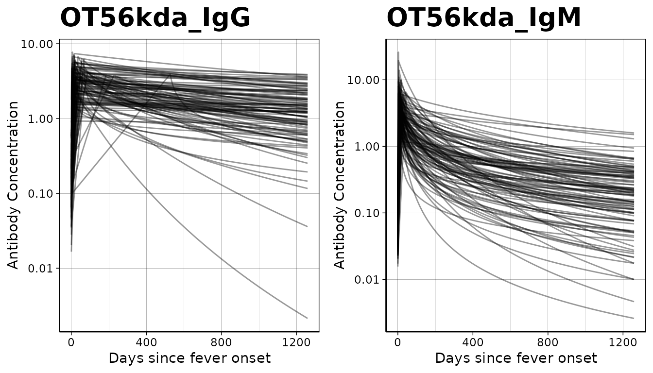

Visualize curve parameters

We can graph the decay curves with an autoplot() method:

curves %>% autoplot()

Load and prepare cross-sectional data

Next, we load our sample cross-sectional data.

# Import cross-sectional data from OSF and rename required variables
xs_data <- load_pop_data(
  file_path = "https://osf.io/download/h5js4/",
  age = "Age",
  value = "result",
  id = "index_id",
  standardize = TRUE
)

Check formatting

We can check that xs_data has the correct formatting using the check_pop_data() function:

xs_data %>% check_pop_data(verbose = TRUE)
#> data format is as expected.

Summarize antibody data

We can compute numerical summaries of our cross-sectional antibody data with a summary() method for pop_data objects:

xs_data %>% summary(strata = "country")
#> Warning: There were 2 warnings in `dplyr::summarize()`.
#> The first warning was:
#> ℹ In argument: `across(...)`.
#> ℹ In group 4: `antigen_iso = OT56kda_IgM` and `country = Nepal`.
#> Caused by warning in `min()`:
#> ! no non-missing arguments to min; returning Inf
#> ℹ Run `dplyr::last_dplyr_warnings()` to see the 1 remaining warning.
#> 
#> n = 1608 
#> 
#> Distribution of age: 
#> 
#> # A tibble: 2 × 8
#>   country     n   min first_quartile median  mean third_quartile   max
#>   <fct>   <int> <dbl>          <dbl>  <dbl> <dbl>          <dbl> <dbl>
#> 1 India     721  18             40     49    50.5           62    87  
#> 2 Nepal     887   0.9            5.5   10.9  11.6           17.0  27.4
#> 
#> Distributions of antigen-isotype measurements:
#> 
#> # A tibble: 4 × 8
#>   antigen_iso country     Min `1st Qu.` Median `3rd Qu.`     Max `# NAs`
#>   <fct>       <fct>     <dbl>     <dbl>  <dbl>     <dbl>   <dbl>   <int>
#> 1 OT56kda_IgG India     0.05      0.111  0.222     2.56     3.81       0
#> 2 OT56kda_IgM India     0.051     0.1    0.139     0.229    3.60       0
#> 3 OT56kda_IgG Nepal     0.112     0.335  0.464     0.602    3.29       0
#> 4 OT56kda_IgM Nepal   Inf        NA     NA        NA     -Inf       1105

Visualize antibody data

Let’s also take a look at how antibody responses change by age.

# Plot antibody responses by age
autoplot(object = xs_data, type = "age-scatter", strata = "Country")
#> Warning: Removed 1105 rows containing missing values or values outside the scale range
#> (`geom_point()`).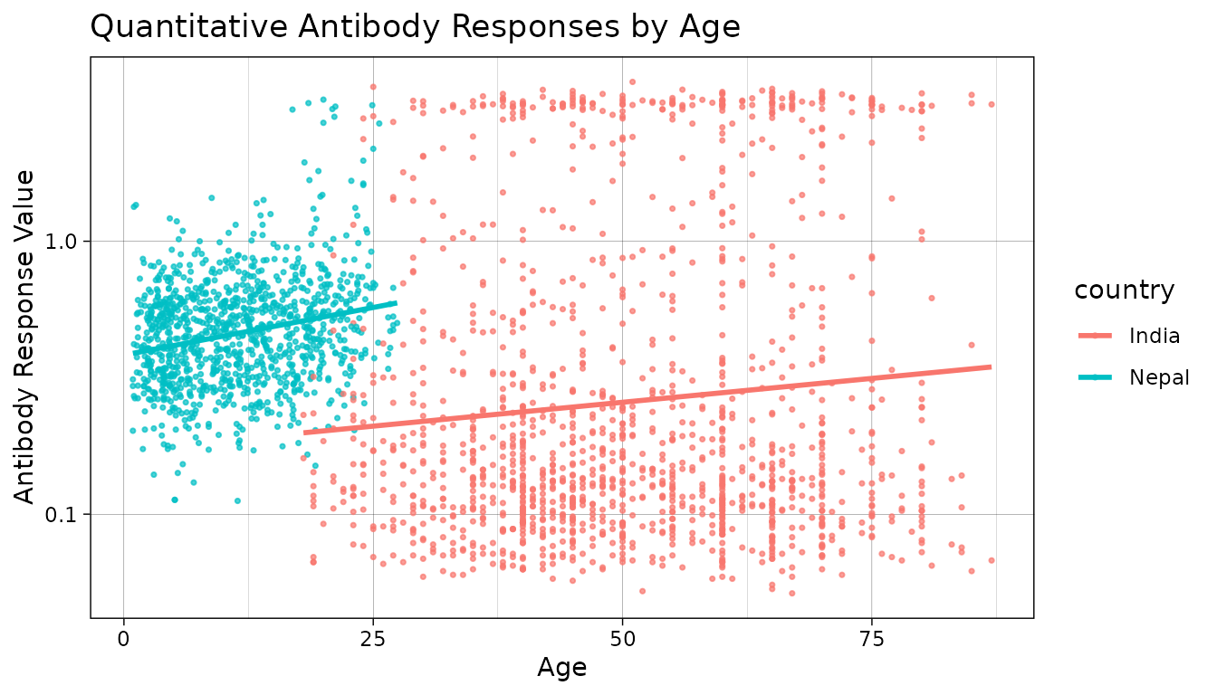

Compile noise parameters

Next, we must set conditions based on some assumptions about the data and errors that may need to be accounted for. This will differ based on background knowledge of the data.

The biological noise, $\nu$ (“nu”), represents error from cross-reactivity to other antibodies. Measurement noise, $\varepsilon$ (“epsilon”), represents error from the laboratory testing process.

Formatting Specifications: Noise parameter data should be a dataframe with one row for each antigen isotype and columns for each noise parameter below.

Column Name	Description
y.low	Lower limit of detection of the antibody assay
nu	Biologic noise
y.high	Upper limit of detection of the antibody assay
eps	Measurement noise

Note that variable names are case-sensitive.

# biologic noise
b.noise <- xs_data %>%
  group_by(antigen_iso) %>%
  filter(!is.na(value)) %>%
  filter(age < 40) %>% # restrict to young ages to capture recent exposures
  do({
    set.seed(54321)
    # Fit the mixture model
    mixmod <- normalmixEM(.$value, k = 2, maxit = 1000) # k is the number of components, adjust as necessary
    # Assuming the first component is the lower distribution
    lower_mu <- mixmod$mu[1]
    lower_sigma <- sqrt(mixmod$sigma[1])
    # Calculate the 90th percentile of the lower distribution
    percentile75 <- qnorm(0.75, lower_mu, lower_sigma)
    # Return the results
    data.frame(antigen_iso = .$antigen_iso[1], percentile75 = percentile75)
  })
#> number of iterations= 35 
#> number of iterations= 24



# define conditional parameters
noise <- data.frame(
  antigen_iso = c("OT56kda_IgG", "OT56kda_IgM"),
  nu = as.numeric(c(b.noise[2, 2], b.noise[1, 2])), # Biologic noise (nu)
  eps = c(0.2, 0.2), # M noise (eps)
  y.low = c(0.2, 0.2), # low cutoff (llod)
  y.high = c(200, 200)
) %>% # high cutoff (y.high)
  mutate(across(where(is.numeric), round, digits = 2))

Estimate Seroincidence by study site

Now we are ready to begin estimating seroincidence. We will use est.incidence.by to calculate stratified seroincidence rates.

# Using est.incidence.by (strata)

est <- est.incidence.by(
  strata = c("country"),
  pop_data = xs_data,
  curve_params = curves,
  noise_params = noise,
  antigen_isos = c("OT56kda_IgG"),
  num_cores = 8 # Allow for parallel processing to decrease run time
)
#> Warning in warn.missing.strata(data = curve_params, strata = strata %>% : curve_params is missing all strata variables, and will be used unstratified.
#> 
#> To avoid this warning, specify the desired set of stratifying variables in the `curve_strata_varnames` and `noise_strata_varnames` arguments to `est.incidence.by()`.
#> Warning in warn.missing.strata(data = noise_params, strata = strata %>% : noise_params is missing all strata variables, and will be used unstratified.
#> 
#> To avoid this warning, specify the desired set of stratifying variables in the `curve_strata_varnames` and `noise_strata_varnames` arguments to `est.incidence.by()`.
#> Warning in check_parallel_cores(.): This computer appears to have 4 cores
#> available. `est.incidence.by()` has reduced its `num_cores` argument to 3 to
#> avoid destabilizing the computer.

summary(est)
#> Seroincidence estimated given the following setup:
#> a) Antigen isotypes   : OT56kda_IgG 
#> b) Strata       : country 
#> 
#>  Seroincidence estimates:
#> # A tibble: 2 × 13
#>   Stratum country     n est.start incidence.rate      SE  CI.lwr CI.upr coverage
#>   <chr>   <fct>   <int>     <dbl>          <dbl>   <dbl>   <dbl>  <dbl>    <dbl>
#> 1 Stratu… India     721       0.1        0.0202  0.00148 0.0175  0.0233     0.95
#> 2 Stratu… Nepal    1105       0.1        0.00854 0.00107 0.00668 0.0109     0.95
#> # ℹ 4 more variables: log.lik <dbl>, iterations <int>, antigen.isos <chr>,
#> #   nlm.convergence.code <ord>

Estimate Seroincidence by study site and age strata

Now we are ready to begin estimating seroincidence. We will use est.incidence.by to calculate stratified seroincidence rates.

# Using est.incidence.by (strata)

est2 <- est.incidence.by(
  strata = c("country", "ageQ"),
  pop_data = xs_data,
  curve_params = curves,
  noise_params = noise,
  antigen_isos = c("OT56kda_IgG"),
  num_cores = 8 # Allow for parallel processing to decrease run time
)
#> Warning in warn.missing.strata(data = curve_params, strata = strata %>% : curve_params is missing all strata variables, and will be used unstratified.
#> 
#> To avoid this warning, specify the desired set of stratifying variables in the `curve_strata_varnames` and `noise_strata_varnames` arguments to `est.incidence.by()`.
#> Warning in warn.missing.strata(data = noise_params, strata = strata %>% : noise_params is missing all strata variables, and will be used unstratified.
#> 
#> To avoid this warning, specify the desired set of stratifying variables in the `curve_strata_varnames` and `noise_strata_varnames` arguments to `est.incidence.by()`.
#> Warning in check_parallel_cores(.): This computer appears to have 4 cores
#> available. `est.incidence.by()` has reduced its `num_cores` argument to 3 to
#> avoid destabilizing the computer.

summary(est2)
#> Seroincidence estimated given the following setup:
#> a) Antigen isotypes   : OT56kda_IgG 
#> b) Strata       : country, ageQ 
#> 
#>  Seroincidence estimates:
#> # A tibble: 5 × 14
#>   Stratum   country ageQ      n est.start incidence.rate      SE  CI.lwr  CI.upr
#>   <chr>     <fct>   <fct> <int>     <dbl>          <dbl>   <dbl>   <dbl>   <dbl>
#> 1 Stratum 1 India   18-29    59       0.1        0.00985 0.00330 0.00511 0.0190 
#> 2 Stratum 2 India   30-49   302       0.1        0.0151  0.00178 0.0120  0.0190 
#> 3 Stratum 3 India   50-89   360       0.1        0.0288  0.00290 0.0236  0.0350 
#> 4 Stratum 4 Nepal   0-17    876       0.1        0.00606 0.00108 0.00428 0.00860
#> 5 Stratum 5 Nepal   18-29   229       0.1        0.0144  0.00259 0.0101  0.0205 
#> # ℹ 5 more variables: coverage <dbl>, log.lik <dbl>, iterations <int>,
#> #   antigen.isos <chr>, nlm.convergence.code <ord>

Let’s visualize our seroincidence estimates by strata.

# Plot seroincidence estimates

# Save summary(est) as a dataframe
estdf <- summary(est) %>%
  mutate(ageQ = "Overall")

# Save summary(est2) as a dataframe
est2df <- summary(est2)


est.comb <- rbind(estdf, est2df)

# Create barplot (rescale incidence rate and CIs)
ggplot(est.comb, aes(y = ageQ, x = incidence.rate * 1000, fill = country)) +
  geom_bar(stat = "identity", position = position_dodge2(width = 0.8, preserve = "single")) +
  geom_linerange(aes(xmin = CI.lwr * 1000, xmax = CI.upr * 1000),
    position = position_dodge2(width = 0.8, preserve = "single")
  ) +
  labs(
    title = "Enteric Fever Seroincidence by Catchment Area",
    x = "Seroincience rate per 1000 person-years",
    y = "Catchment"
  ) +
  theme_bw() +
  facet_wrap(~country) +
  theme(
    axis.text.y = element_text(size = 11),
    axis.text.x = element_text(size = 11)
  ) +
  scale_fill_manual(values = c("orange2", "#39558CFF", "red"))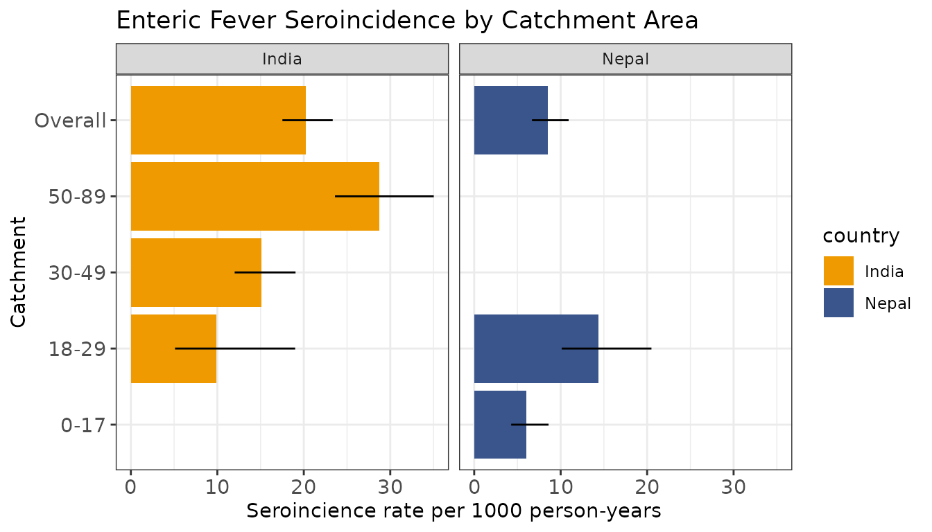

Acknowledgments

We gratefully acknowledge the study participants for their valuable time and interest in participating in these studies

Funding

This work was supported by the National Institutes of Health Fogarty International Center (FIC) at [K01 TW012177] and the National Institute of Allergy and Infectious Diseases (NIAID) [R21 1AI176416]

References

Aiemjoy, K, N Katuwal, K Vaidya, S Shrestha, M Thapa, PFM Teunis, II Bogoch, et al. Accepted Feb 2024. “Estimating the Seroincidence of Scrub Typhus Using Antibody Dynamics Following Infection.” American Journal of Tropical Medicine and Hygiene, Accepted Feb 2024.

deGraaf, WF, MEE Kretzschmar, PFM Teunis, and O Diekmann. 2014. “A Two-Phase Within-Host Model for Immune Response and Its Application to Serological Profiles of Pertussis.” Epidemics 9 (December): 1–7. https://doi.org/10.1016/j.epidem.2014.08.002.

Simonsen, J, K Mølbak, G Falkenhorst, KA Krogfelt, A Linneberg, and PFM Teunis. 2009. “Estimation of Incidences of Infectious Diseases Based on Antibody Measurements.” Statistics in Medicine 28 (14): 1882–95. https://doi.org/10.1002/sim.3592.

Teunis, PFM, and JCH van Eijkeren. 2020. “Estimation of Seroconversion Rates for Infectious Diseases: Effects of Age and Noise.” Statistics in Medicine 39 (21): 2799–2814. https://doi.org/10.1002/sim.8578.

Teunis, PFM, JCH van Eijkeren, CW Ang, YTHP van Duynhoven, JB Simonsen, MA Strid, and W van Pelt. 2012. “Biomarker Dynamics: Estimating Infection Rates from Serological Data.” Statistics in Medicine 31 (20): 2240–48. https://doi.org/10.1002/sim.5322.

Teunis, PFM, JCH van Eijkeren, WF deGraaf, A Bonačić Marinović, and MEE Kretzschmar. 2016. “Linking the Seroresponse to Infection to Within-Host Heterogeneity in Antibody Production.” Epidemics 16 (September): 33–39. https://doi.org/10.1016/j.epidem.2016.04.001.

UC Davis Seroepidemiology Research Group (SERG)