Attaching package: 'dplyr'The following objects are masked from 'package:stats':
filter, lagThe following objects are masked from 'package:base':
intersect, setdiff, setequal, unionInvalid Date
The incidence rate of a disease over a specific time period is the rate at which individuals in a population are acquiring the disease during that time period (Noordzij et al. 2010).
Example: if there are 10 new cases of typhoid in a population of 1000 persons during a one month time period, then the incidence rate for that time period is 10 new cases per 1000 persons per month.
More mathematically, the incidence rate at a given time point is the derivative (i.e., the current rate of change over time) of the expected cumulative count of infections per person at risk, at that time:
\[\frac{d}{dt} \mathbb{E}\left[\frac{C(t)}{n} \mid N(t) =n\right]\]
where \(C(t)\) is the cumulative total number of infections in the population of interest, and \(N(t)\) is the number of individuals at risk at time \(t\).
In both definitions, the units for an incidence rate are “# new infections per # persons at risk per time duration”; for example, “new infections per 1000 persons per year”.
For convenience, we can rescale the incidence rate to make it easier to understand; for example, we might express incidence as “# new infections per 1000 persons per year” or “# new infections per 100,000 persons per day”, etc.
From the perspective of an individual in the population:
the incidence rate (at a given time point (\(t\)) is the instantaneous probability (density) of becoming infected at that time point, given that they are at risk at that time point.
That is, the incidence rate is a hazard rate.
Notation: let’s use \(\lambda_{t}\) to denote the incidence rate at time \(t\).
Typically, it is difficult to estimate changes from a single time point. However, we can sometimes make assumptions that allow us to do so. In particular, if we assume that the incidence rate is constant over time, then we can estimate incidence from a single cross-sectional survey.
We will need two pieces of notation to formalize this process.
We recruit participants from the population of interest.
For each survey participant, we measure antibody levels \((Y)\) for the disease of interest
Each participant was most recently infected at some time \((T)\) prior to when we measured their antibodies.
We assume that:
(We can analyze subpopulations separately to make homogeneity more plausible.)
(For diseases like typhoid, the no-immunity assumption may not hold exactly, but hopefully approximately; modeling the effects of re-exposure during an active infection is on our to-do list).
Under those assumptions:
\[\mathbb{p}(T=t) = \lambda \exp{\left\{-\lambda t\right\}}\]
\[\mathbb{p}(T=t|A=a) = 1_{t \in[0,a]}\lambda \exp{\left\{-\lambda t\right\}} + 1_{t = \text{NA}} \exp{\left\{-\lambda a\right\}}\]
This is a time-to-event model, looking backwards in time from the survey date (when the blood sample was collected).
The probability that an individual was last infected \(t\) days ago, \(p(T=t)\), is equal to the probability of being infected at time \(t\) (i.e., the incidence rate at time \(t\), \(\lambda\)) times the probability of not being infected after time \(t\), which turns out to be \(\exp(-\lambda t)\).
The distribution of \(T\) is truncated by the patient’s birth date; the probability that they have never been infected is \(\exp{\left\{-\lambda a\right\}}\), where \(a\) is the patient’s age at the time of the survey.
If we could observe \(T\), then we could estimate \(\lambda\) using a typical maximum likelihood approach.
Starting with the likelihood: Taking the logarithm of the likelihood: Taking the derivative of that log-likelihood to find the score function: Setting the score function equal to 0 to find the score equation, and solving the score equation for \(\lambda\) to find the maximum likelihood estimate:
\[\mathcal{L}^*(\lambda) = \prod_{i=1}^n \mathbb{p}(T=t_i) = \prod_{i=1}^n \lambda \exp(-\lambda t_i)\]
\[\ell^*(\lambda) = \log{\left\{\mathcal{L}^*(\lambda)\right\}} = \sum_{i=1}^n \log{\left\{\lambda\right\}} -\lambda t_i\]
\[\ell^{*'}(\lambda) = \sum_{i=1}^n \lambda^{-1} - t_i\]
\[\hat{\lambda}_{\text{ML}} = \frac{n}{\sum_{i=1}^n t_i} = \frac{1}{\bar{t}}\]
The MLE turns out to be the inverse of the mean.
Here’s what that would look like:
Attaching package: 'dplyr'The following objects are masked from 'package:stats':
filter, lagThe following objects are masked from 'package:base':
intersect, setdiff, setequal, union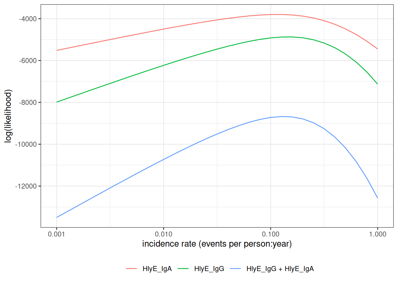
The standard error of the estimate is approximately equal to the inverse of the rate of curvature (2nd derivative, aka Hessian) in the log-likelihood function, at the maximum:
more curvature -> likelihood peak is clearer -> smaller standard errors
Unfortunately, we don’t observe infection times \(T\); we only observe antibody levels \({Y}\). So things get a little more complicated.
In short, we are hoping that we can estimate \(T\) (time since last infection) from \(Y\) (current antibody levels). If we could do that, then we could plug in our estimates \(\hat t_i\) into that likelihood above, and estimate \(\lambda\) as previously.
We’re actually going to do something a little more nuanced; instead of just using one value for \(\hat t\), we are going to consider all possible values of \(t\) for each individual.
We need to link the data we actually observed to the incidence rate.
The likelihood of an individual’s observed data, \(\mathbb{p}(Y=y)\), can be expressed as an integral over the joint likelihood of \(Y\) and \(T\) (using the Law of Total Probability):
Further, we can express the joint probability \(p(Y=y,T=t)\) as the product of \(p(T=t)\) and \(p(Y=y|T=t)\) the “antibody response curve after infection”. That is:

Substituting \(p(Y=y,T=t) = p(Y=y|T=t)P(T=t)\) into the previous expression for \(p(Y=y)\):
\[ \begin{aligned} p(Y=y) &= \int_t p(Y=y|T=t)P(T=t) dt \end{aligned} \]
Now, the likelihood of the observed data \(\mathbf{y} = (y_1, y_2, ..., y_n)\) is:
\[ \begin{aligned} \mathcal{L}(\lambda) &= \prod_{i=1}^n p(Y=y_i) \\&= \prod_{i=1}^n \int_t p(Y=y_i|T=t)p_\lambda(T=t)dt\\ \end{aligned} \]
If we know \(p(Y=y|T=t)\), then we can maximize \(\mathcal{L}(\lambda)\) over \(\lambda\) to find the “maximum likelihood estimate” (MLE) of \(\lambda\), denoted \(\hat\lambda\).
The likelihood of \(Y\) involves the product of integrals, so the log-likelihood involves the sum of the logs of integrals:
\[ \begin{aligned} \log \mathcal{L} (\lambda) &= \log \prod_{i=1}^n \int_t p(Y=y_i|T=t)p_\lambda(T=t)dt\\ &= \sum_{i=1}^n \log\left\{\int_t p(Y=y_i|T=t)p_\lambda(T=t)dt\right\}\\ \end{aligned} \]
The derivative of this expression doesn’t come out cleanly, so we will use a numerical method (specifically, a Newton-type algorithm, implemented by stats::nlm()) to find the MLE and corresponding standard error.
In many survey designs, observations are clustered (e.g., multiple individuals from the same household, school, or geographic area). Observations within the same cluster are often more similar to each other than to observations from different clusters, violating the independence assumption of standard maximum likelihood estimation.
When observations are clustered:
To account for within-cluster correlation, serocalculator implements the sandwich estimator (also known as the Huber-White robust variance estimator):
\[V_{\text{robust}} = H^{-1} B H^{-1}\]
where:
\[B = \sum_{c=1}^C U_c U_c^T\]
where:
Users can specify clustering using the cluster_var parameter:
When cluster-robust standard errors are used, the summary() output indicates this with se_type = "cluster-robust".
Now, we need a model for the antibody response to infection, \(\mathbb{p}(Y=y|T=t)\). The current version of the serocalculator package uses a two-phase model for the shape of the seroresponse (Teunis et al. 2016).
The first phase of the model represents the active infection period, and uses a simplified Lotka-Volterra predator-prey model (Volterra 1928) where the pathogen is the prey and the antibodies are the predator:
Notation:
Model:
With baseline antibody concentration \(y(0) = y_{0}\) and initial pathogen concentration \(x(0) = x_{0}\).
Compared to the standard LV model:
the predation term with the \(\beta\) coefficient is missing the prey concentration \(x(t)\) factor; we assume that the efficiency of predation doesn’t depend on pathogen concentration.
the differential equation for predator density is missing the predator death rate term \(-\gamma y(t)\); we assume that as long as there are any pathogens present, the antibody decay rate is negligible compared to the growth rate.
the predator growth rate term \(\delta y(t)\) is missing the prey density factor \(x(t)\) we assume that as long as there are any pathogens present, the antibody concentration grows at the same exponential rate.
These omissions were made to simplify the estimation process, under the assumption that they are negligible compared to the other terms in the model.
\[b(t) = 0\]
\[y^{\prime}(t) = -\alpha y(t)^r\]
Antibody decay is different from exponential (log–linear) decay. When the shape parameter \(r > 1\), log concentrations decrease rapidly after infection has terminated, but decay then slows down and low antibody concentrations are maintained for a long period. If \(r = 1\), this model reduces to exponential decay with decay rate \(\alpha\).
The serum antibody response \(y(t)\) can be written as
\[ y(t) = y_{+}(t) + y_{-}(t) \]
where
\[ \begin{align} y_{+}(t) & = y_{0}\text{e}^{\mu t}[0\leq t <t_{1}]\\ y_{-}(t) & = y_{1}\left(1+(r-1)y_{1}^{r-1}\alpha(t-t_{1})\right)^{-\frac{1}{r-1}}[t_{1}\le t < \infty] \end{align} \]
Since the peak level is \(y_{1} = y_{0}\text{e}^{\mu t_{1}}\) the growth rate \(\mu\) can be written as \[\mu = \frac{1}{t_{1}}\log\left(\frac{y_{1}}{y_{0}}\right)\]
Scale for x is already present.
Adding another scale for x, which will replace the existing scale.
Warning: Computation failed in `stat_function()`.
Caused by error in `if (r == 1) ...`:
! argument is of length zero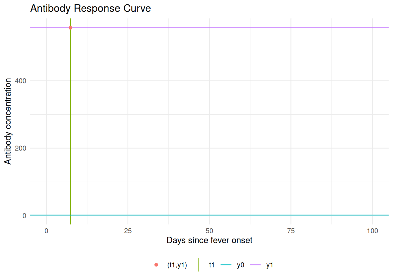
The antibody level at \(t=0\) is \(y_{0}\); the rising branch ends at \(t = t_{1}\) where the peak antibody level \(y_{1}\) is reached. Any antibody level \(y(t) \in (y_{0}, y_{1})\) eventually occurs twice.
An interactive Shiny app that allows the user to manipulate the model parameters is available at:

When we measure antibody concentrations in a blood sample, we are essentially counting molecules (using biochemistry).
We might miss some of the antibodies (undercount, false negatives) and we also might incorrectly count some other molecules that aren’t actually the ones we are looking for (overcount, false positives, cross-reactivity).
We are more concerned about overcount (cross-reactivity) than undercount. For a given antibody, we can do some analytical work beforehand to estimate the distribution of overcounts, and add that to our model \(p(Y=y|T=t)\).
Notation:
Model:
\(\nu\) needs to be pre-estimated using negative controls, typically using the 95th percentile of the distribution of antibody responses to the antigen-isotype in a population with no exposure.
There are also some other sources of noise in our bioassays; user differences in pipetting technique, random ELISA plate effects, etc. This noise can cause both overcount and undercount. We can also estimate the magnitude of this noise source and include it in \(p(Y=y|T=t)\).
Measurement noise, \(\varepsilon\) (“epsilon”), represents measurement error from the laboratory testing process. It is defined by a CV (coefficient of variation) as the ratio of the standard deviation to the mean for replicates. Note that the CV should ideally be measured across plates rather than within the same plate.