6 R Coding Practices
6.1 Lab Protocols for Code and Data
Just as wet labs have strict safety protocols to ensure reproducible results and prevent contamination, our computational lab has protocols for coding and data management. These protocols are not suggestions—they are essential practices that:
- Ensure reproducibility: Others (including your future self) can recreate your analysis
- Prevent errors: Systematic approaches reduce the risk of mistakes
- Enable collaboration: Consistent practices allow team members to work together efficiently
- Maintain data integrity: Proper handling prevents data corruption and loss
- Support publication: Well-documented, reproducible code is increasingly required for publication
Violating these protocols can have serious consequences, including invalid results, wasted time, inability to publish, and damage to scientific credibility. Treat coding and data management protocols with the same seriousness as you would safety protocols in a wet lab.
6.2 The Tool-Building Mindset
A tool is anything that makes a task easier when that task would otherwise be repetitive, hard, or impossible — a script, a function, a package, a spreadsheet, a checklist, or a CI workflow. Aaron Crosman’s Tool Building Mindset argues for taking that expansive view deliberately: everyone who works with technology should, can, and already does build tools for themselves, whether or not they think of themselves as a “developer.”
The mindset in practice:
- Notice the friction. When you catch yourself repeating a task, following a fragile manual sequence, or avoiding something because it is tedious, treat that as a signal to build (or find) a tool for it.
- Look before you build — then chip away. Check whether an existing tool already solves the problem (see Section 7.5); when nothing quite fits, don’t let “not worth the effort” stop you: a tool that removes part of an annoying task is already good enough to start with.
- Start small and grow the tool as it earns it. A copy-pasted snippet becomes a function; a function used across analyses becomes a package (see Section 6.4); a workflow copied between repositories becomes a shared, reusable one.
- Build for your own repeated use first. A tool that saves you an hour a week justifies itself quickly, and the discipline of packaging it (documentation, tests) makes it usable by the next lab member too.
- Don’t gold-plate. The tool only needs to beat doing the task by hand; polish it further only when its use grows to warrant it.
Much of our lab’s shared infrastructure came from exactly this pattern: the {snapr} package packages the lab’s snapshot-testing helpers, the {lms} linter package packages our shared lint configuration, and the d-morrison/gha repository collects reusable CI workflows and composite actions shared across the lab’s repositories.
6.3 Essential R Package Development Tools
The following tools are essential for R package development in our lab:
6.3.1 usethis: Package Setup and Management
usethis automates common package development tasks:
# Install usethis
install.packages("usethis")

# Create a new package
usethis::create_package("~/myproject")

# Add common components
usethis::use_mit_license()          # Add a license
usethis::use_git()                  # Initialize git
usethis::use_github()               # Connect to GitHub
usethis::use_testthat()             # Set up testing infrastructure
usethis::use_vignette("intro")      # Create a vignette (shipped with package)
usethis::use_article("case-study")  # Create an article (website-only)
usethis::use_data_raw("dataset")    # Create data processing script
usethis::use_package("dplyr")       # Add a dependency
usethis::use_pipe()                 # Import magrittr pipe operator (no longer recommended)

# Increment version
usethis::use_version()              # Increment package version
6.3.2 devtools: Development Workflow
devtools provides the core development workflow:
# Install devtools
install.packages("devtools")

# Load your package for interactive development
devtools::load_all()                # Like library(), but for development

# Documentation
devtools::document()                # Generate documentation from roxygen2

# Testing
devtools::test()                    # Run all tests
devtools::test_active_file()        # Run tests in current file

# Checking
devtools::check()                   # R CMD check (comprehensive validation)
devtools::check_man()               # Check documentation only

# Dependencies
devtools::install_dev_deps()        # Install all development dependencies

# Building
devtools::build()                   # Build package bundle
devtools::install()                 # Install package locally
6.3.3 pkgdown: Package Websites
pkgdown builds beautiful documentation websites from your package:
# Install pkgdown
install.packages("pkgdown")

# Set up pkgdown
usethis::use_pkgdown()

# Build website locally
pkgdown::build_site()

# Preview in browser
pkgdown::build_site(preview = TRUE)

# Build components separately
pkgdown::build_reference()          # Function reference
pkgdown::build_articles()           # Vignettes
pkgdown::build_home()               # Home page from README
Configure your pkgdown site with _pkgdown.yml:
url: https://ucd-serg.github.io/YOURPROJECT

template:
  bootstrap: 5

reference:
  - title: "Data Preparation"
    desc: "Functions for preparing and cleaning data"
    contents:
    - prep_study_data
    - validate_data

  - title: "Analysis"
    desc: "Core analysis functions"
    contents:
    - run_primary_analysis
    - sensitivity_analysis

articles:
  - title: "Analysis Workflow"
    navbar: Analysis
    contents:
    - 01-data-preparation
    - 02-primary-analysis
    - 03-sensitivity-analysis
6.3.4 Alternatives to pkgdown
While {pkgdown} is the standard tool for creating package documentation websites, several alternatives exist that may better suit specific needs, particularly for generating multiple output formats beyond HTML.
6.3.4.1 altdoc
{altdoc} is a flexible alternative that supports multiple documentation frameworks, including Quarto, Docsify, MkDocs, and Docute. It is especially useful when you need to generate documentation in multiple formats.
Key features:
- Supports multiple documentation frameworks (Quarto, Docsify, MkDocs, Docute)
- Renders Quarto and R Markdown vignettes to HTML websites
- When using Quarto as the framework, vignettes can be authored to support multiple output formats (HTML, PDF, DOCX, reveal.js presentations), and Quarto can include download links for alternative formats on the HTML site (see Quarto documentation on multiple formats)
- Handles function reference pages, README, NEWS, and other standard documentation
- Easy preview and deployment workflow
Basic usage:
# Install altdoc
install.packages("altdoc")

# Set up documentation with Quarto
altdoc::setup_docs(tool = "quarto_website")

# Or use other frameworks
# altdoc::setup_docs(tool = "docsify")
# altdoc::setup_docs(tool = "mkdocs")
# altdoc::setup_docs(tool = "docute")

# Render documentation
altdoc::render_docs()

# Preview in browser
altdoc::preview_docs()
When to choose altdoc:
- You want to use Quarto’s modern publishing system for your documentation website
- You need vignettes that can be downloaded in multiple formats (when authored with Quarto’s multi-format support)
- You prefer a different documentation framework than pkgdown’s Bootstrap-based approach (Docsify, MkDocs, or Docute)
- You need more flexibility in site design and structure
6.3.4.2 pkgsite
{pkgsite} provides a minimal, lightweight alternative to pkgdown, focusing on simplicity and ease of customization.
Key features:
- Minimal CSS framework (no Bootstrap)
- Simple, clean design that is easy to customize
- Similar
build_site()function to pkgdown - Lightweight and fast
- Can be published via GitHub Pages or other static site hosts
Basic usage:
# Install pkgsite (not on CRAN as of early 2026)
pak::pkg_install("pachadotdev/pkgsite")

# Build and preview site
pkgsite::build_site(preview = TRUE)

# Build with custom URL and lazy rebuilding
pkgsite::build_site(
  # Replace with your real docs domain.
  url = "https://example.com",
  lazy = TRUE,
  preview = TRUE
)
When to choose pkgsite:
- You want a minimal, lightweight documentation site
- You prefer to customize CSS styling from scratch
- You don’t need the extensive features of pkgdown
- You want faster build times for simple packages
6.3.4.3 Quarto for Package Documentation
While not a dedicated package documentation tool, Quarto can be used to create sophisticated documentation websites for R packages, particularly when combined with custom scripts or tools like {ecodown} (experimental and intended for internal use).
Discussion and resources:
- Quarto discussion on pkgdown alternative
- pkgdown itself now supports Quarto vignettes (as of version 2.1.0)
When to consider Quarto:
- You want complete control over site structure and design
- You’re already using Quarto for other documentation
- You need advanced publishing features beyond what pkgdown offers
- You’re comfortable writing custom scripts for function reference extraction
6.3.4.4 Comparison Summary
| Tool | Complexity | Website Output | Multi-format Support | Customization | Best For |
|---|---|---|---|---|---|
| pkgdown | Standard | HTML | Limited (via Quarto vignettes) | Template-based | Most R packages, standard documentation needs |
| altdoc | Moderate | HTML | Yes (via Quarto-authored vignettes with download links) | Framework-dependent | Quarto-based workflows, flexible frameworks |
| pkgsite | Minimal | HTML | No | High (simple CSS) | Lightweight sites, custom styling |
| Quarto | Advanced | HTML (for websites) | Yes (native - can output to PDF, DOCX, reveal.js, EPUB) | Complete | Full control, advanced features |
Recommendation: Use pkgdown for most standard R package documentation needs. Consider altdoc when you prefer Quarto’s publishing system or want flexibility to choose between documentation frameworks (Quarto, Docsify, MkDocs, Docute). If you choose altdoc with Quarto, you can author vignettes to provide downloadable PDF and DOCX versions alongside the HTML website. Choose pkgsite for minimalist websites with easy CSS customization. Use Quarto directly only if you need complete control and are comfortable with more complex setup.
6.4 Complete Package Development Workflow
Here’s the typical workflow for developing an R package in our lab:
6.4.1 1. Initial Setup
Starting from a template (recommended):
Using our R package template is the fastest way to get started with a new R package, as it provides pre-configured settings, GitHub Actions workflows, and development tools:
- UCD-SeRG R Package Template - Our recommended template with pre-configured development tools and CI workflows:
- Repository: https://github.com/UCD-SERG/rpt
- Click “Use this template” → “Create a new repository” on GitHub
- Clone your new repository and start developing
The template includes pre-configured:
- GitHub Actions workflows for R CMD check, test coverage, and pkgdown deployment
- Development tools setup (
{usethis},{devtools},{roxygen2}) - Testing infrastructure (
{testthat}) - Code styling and linting configurations
- Package documentation structure
While the template jumpstarts your project with up-to-date configuration and workflow files, you should still come up to speed on what all the config files do so you can modify and debug them as needed. The template serves as a central location for the most current versions of these files and best practices.
Starting from scratch:
If you prefer to start from scratch or need to understand each setup step, you can create a new package manually:
# Create package structure
usethis::create_package("~/myproject")

# Set up infrastructure
usethis::use_git()
usethis::use_github()
usethis::use_testthat()
usethis::use_pkgdown()
usethis::use_mit_license()
usethis::use_readme_rmd()
6.4.2 2. Add Dependencies
# Add packages your project depends on
usethis::use_package("dplyr")
usethis::use_package("ggplot2")
usethis::use_package("readr")

# Add packages only needed for development/testing
usethis::use_package("testthat", type = "Suggests")
6.4.3 3. Write Functions
Create functions in R/ directory with roxygen2 documentation:
#' Prepare Study Data
#'
#' Clean and prepare raw study data for analysis.
#'
#' @param raw_data A data frame containing raw study data
#' @param validate Logical; whether to run validation checks
#'
#' @returns A cleaned data frame ready for analysis
#'
#' @examples
#' raw_data <- read_csv("data.csv")
#' clean_data <- prep_study_data(raw_data)
#'
#' @export
prep_study_data <- function(raw_data, validate = TRUE) {
  # Function implementation
}
6.4.4 4. Document
# Generate documentation from roxygen2 comments
devtools::document()
6.4.5 5. Test
Create tests in tests/testthat/:
# tests/testthat/test-data_prep.R
test_that("prep_study_data handles missing values", {
  raw_data <- data.frame(x = c(1, NA, 3))
  result <- prep_study_data(raw_data)
  expect_false(anyNA(result$x))
})
Run tests:
devtools::test()6.4.6 6. Check
# Comprehensive package check
devtools::check()
Fix any warnings or errors before proceeding.
6.4.7 7. Build Documentation Site
pkgdown::build_site()6.5 Organizing scripts
Just as your data “flows” through your project, data should flow naturally through a script. Very generally, you want to:
- describe the work completed in the script in a comment header
- source your configuration file (
0-config.R) - load all your data
- do all your analysis/computation
- save your data.
Each of these sections should be “chunked together” using comments. See this file for a good example of how to cleanly organize a file in a way that follows this “flow” and functionally separate pieces of code that are doing different things.
6.6 Testing Requirements
ALWAYS establish tests BEFORE modifying functions. This ensures changes preserve existing behavior and new behavior is correctly validated.
6.6.1 When to Use Snapshot Tests
Use snapshot tests (expect_snapshot(), expect_snapshot_value()) when:
- Testing complex data structures (data frames, lists, model outputs)
- Validating statistical results where exact values may vary slightly
- Output format stability is important
test_that("prep_study_data produces expected structure", {
  result <- prep_study_data(raw_data)
  expect_snapshot_value(result, style = "serialize")
})
Our lab’s {snapr} package (on CRAN) adds convenience wrappers on top of {testthat}’s snapshot functions: expect_snapshot_data() for data frames (adapted, with permission, from the {ssdtools} package) and expect_snapshot_object(), which generalizes it to any R object.
test_that("prep_study_data output is stable", {
  result <- prep_study_data(raw_data)
  snapr::expect_snapshot_data(result, name = "prepped_study_data")
})
6.6.2 When to Use Explicit Value Tests
Use explicit tests (expect_equal(), expect_identical()) when:
- Testing simple scalar outputs
- Validating specific numeric thresholds
- Testing Boolean returns or categorical outputs
test_that("calculate_mean returns correct value", {
  expect_equal(calculate_mean(c(1, 2, 3)), 2)
  expect_equal(calculate_ratio(3, 7), 0.4285714, tolerance = 1e-6)
})
6.6.3 Choosing Between Snapshot and Explicit Tests
The two styles answer different questions. A snapshot test asks “does this output still match what it looked like before?”; an explicit test asks “does this specific property equal this exact value?”. That difference drives every practical trade-off, as Table 6.1 summarizes:
| Snapshot test | Explicit test | |
|---|---|---|
| Conciseness | High: one snapshot call pins the whole output, standing in for a long list of assertions, and the first run records the reference automatically | Lower: you write an assertion per property you care about, which adds up fast for complex outputs |
| Readability | Lower: the test shows that output is pinned, not why | Higher: each assertion documents an intended behavior |
| When output legitimately changes | One review-and-accept of the new snapshot | Rewrite the affected assertions by hand |
| Failure diagnosis | A diff of the whole output; the relevant change may be buried | Points at the exact property that broke |
Each style has a characteristic failure mode to guard against:
- Snapshot blindness. Because a snapshot diff can be long, it is tempting to accept an updated snapshot without reading it — which silently converts a regression into the new expected output. Treat every
testthat::snapshot_accept()like a code review: read the diff (testthat::snapshot_review()) before accepting. - Brittle snapshots. Non-deterministic output (timestamps, random numbers, file paths) makes a snapshot fail on every run; seed or fix the inputs first (see the seeding advice under Section 6.6.4).
- Assertion sprawl. Explicitly asserting every field of a large object takes a page of fragile code — exactly the case where one snapshot is clearer.
- Over-specified assertions. Explicit tests pinned to incidental details (element order that doesn’t matter, formatting) fail on harmless refactors and train you to distrust them.
In practice the strongest suites combine both: explicit assertions pin the core logic (the value a calculation must produce, the condition an input must trigger), and a snapshot guards the surrounding large structure (the full prepared data frame, a printed summary) against unnoticed drift. The {testthat} snapshotting vignette covers the workflow — recording, reviewing, and accepting snapshots — in more depth.
6.6.4 Testing Best Practices
- Seed randomness: Use
withr::local_seed()for reproducible tests - Use small test cases: Keep tests fast
- Test edge cases: Missing values, empty inputs, boundary conditions
- Test errors: Verify functions fail appropriately with invalid input
test_that("prep_study_data handles edge cases", {
  # Empty input
  expect_error(prep_study_data(data.frame()))

  # Missing required columns
  expect_error(prep_study_data(data.frame(x = 1)))

  # Valid input with missing values
  result <- prep_study_data(data.frame(id = 1:3, value = c(1, NA, 3)))
  expect_true(all(!is.na(result$value)))
})
6.7 Test-Driven Development
Test-driven development (TDD) inverts the usual order of coding and testing: you write the test for a behavior before writing the code that implements it. The practice was popularized by Kent Beck, who developed it as part of extreme programming and described it in Test-Driven Development: By Example (2002).
Work proceeds in a short, repeated cycle (often called red-green-refactor):
- Red. Write a small test for the next behavior you want, and run it to confirm it fails — this proves the test can actually detect the missing behavior.
- Green. Write the simplest code that makes the test pass, resisting the urge to build ahead of the tests.
- Refactor. Clean up the code (and the tests) while everything stays green, leaning on the tests to catch anything the cleanup breaks.
Why it helps:
- The test pins down what the function should do before you are invested in what it happens to do, turning requirements into executable checks.
- Every unit of behavior ends up covered by construction, so later changes get regression protection for free.
- Code written to be testable tends toward small, single-purpose functions with explicit inputs and outputs — the same design our function-decomposition
- guidance pushes toward.
You do not have to practice strict TDD to benefit from it. Our testing guidance (Section 6.6) already applies its core move — establish tests before modifying existing functions — and writing the test first is just that same discipline applied to new code as well. In R packages, the mechanics are light: usethis::use_test() creates the matching {testthat} test file, and devtools::test() runs the suite (see R Packages, ch. “Testing basics”).
6.8 Benchmarking
This section draws from the Measuring Performance and Improving Performance chapters in Advanced R by Hadley Wickham, along with documentation for {bench} and {profvis}.
Performance optimization starts with measurement. Benchmarking helps identify bottlenecks, compare alternative implementations, and ensure your code meets performance requirements. This section covers when and how to benchmark R code, with a focus on integration with package development workflows.
6.8.1 When to Benchmark
Benchmark when:
- Choosing between implementations: Compare different approaches to the same problem
- Optimizing critical paths: Identify and improve performance bottlenecks
- Preventing regressions: Ensure new code doesn’t slow down existing functionality
- Processing large datasets: Verify scalability for biostatistics/epidemiology workflows
- Implementing computational methods: Test algorithms involving bootstrapping, simulation, or resampling
Don’t benchmark prematurely. Write correct, readable code first, then measure to find what actually needs optimization.
6.8.2 Setting Up Benchmarking Infrastructure
Organize benchmarking code separately from unit tests:
mypackage/
  tests/
    testthat/          # Unit tests (run by R CMD check)
    benchmarks/        # Benchmarking scripts (run manually or in CI)
      01-data-prep.R
      02-analysis.R
Add benchmarking dependencies to DESCRIPTION:
# Add bench and profvis as development dependencies
usethis::use_package("bench", type = "Suggests")
usethis::use_package("profvis", type = "Suggests")

# Add any packages used in benchmarks
# For example, if comparing with data.table or gbm:
# usethis::use_package("data.table", type = "Suggests")
# usethis::use_package("gbm", type = "Suggests")
Create a benchmark template:
# tests/benchmarks/01-data-prep.R
library(bench)
library(mypackage)

# Generate test data
n <- 10000
test_data <- data.frame(
  id = 1:n,
  exposure = rnorm(n),
  outcome = rbinom(n, 1, 0.3)
)

# Compare implementations
results <- bench::mark(
  original = prep_data_v1(test_data),
  optimized = prep_data_v2(test_data),
  check = FALSE,  # Set TRUE to verify outputs are identical
  iterations = 100,
  time_unit = "ms"
)

print(results)
6.8.3 Using bench for Performance Comparisons
{bench} provides accurate performance measurements and makes it easy to compare multiple implementations.
Basic usage:
library(bench)

# Compare different approaches
results <- bench::mark(
  base_subset = data[data$group == "treatment", ],
  dplyr_filter = dplyr::filter(data, group == "treatment"),
  data.table = dt[group == "treatment"],
  iterations = 100
)

# View results
print(results)
#> # A tibble: 3 × 6
#>   expression        min   median `itr/sec` mem_alloc `gc/sec`
#>   <bch:expr>   <bch:tm> <bch:tm>     <dbl> <bch:byt>    <dbl>
#> 1 base_subset    1.2ms    1.4ms       714.    1.5MB     2.14
#> 2 dplyr_filter   2.1ms    2.3ms       435.    2.1MB     4.35
#> 3 data.table   850.0µs  950.0µs      1053.  800.0KB     0.00

# Plot results
plot(results)
Key features:
- Accurate timing: Accounts for overhead and runs multiple iterations
- Memory tracking: Shows memory allocation for each approach
- Garbage collection: Reports GC frequency
- Output verification: Optional checking that all implementations produce identical results
Example for biostatistics workflow:
# Compare propensity score estimation methods
library(bench)

# Simulate cohort data
n <- 5000
cohort <- data.frame(
  age = rnorm(n, 50, 15),
  bmi = rnorm(n, 27, 5),
  treatment = rbinom(n, 1, 0.5),
  outcome = rbinom(n, 1, 0.3)
)

# Note: Install gbm first if not already installed
# usethis::use_package("gbm", type = "Suggests")

# Compare GLM vs GBM for propensity scores
ps_benchmark <- bench::mark(
  glm_method = {
    model <- glm(treatment ~ age + bmi,
                 data = cohort,
                 family = binomial())
    predict(model, type = "response")
  },
  gbm_method = {
    model <- gbm::gbm(treatment ~ age + bmi,
                      data = cohort,
                      distribution = "bernoulli",
                      n.trees = 100,
                      verbose = FALSE)
    predict(model, n.trees = 100, type = "response")
  },
  check = FALSE,
  iterations = 50
)

print(ps_benchmark)
6.8.4 Using profvis for Memory and CPU Profiling
{profvis} identifies where your code spends time and allocates memory. Use it to find bottlenecks in existing functions.
Basic usage:
library(profvis)

# Profile a function
profvis({
  data <- prep_study_data(raw_data)
  results <- run_primary_analysis(data)
})
The profvis output shows:
- Flame graph: Visual representation of time spent in each function
- Data view: Line-by-line time and memory usage
- Memory profile: Allocation patterns over time
Example for data preparation:
library(profvis)

profvis({
  # Profile data cleaning pipeline
  cleaned <- raw_data |>
    dplyr::filter(!is.na(id)) |>
    dplyr::mutate(
      age_group = cut(age, breaks = c(0, 18, 65, Inf)),
      bmi_category = cut(bmi, breaks = c(0, 18.5, 25, 30, Inf))
    ) |>
    dplyr::left_join(exposure_data, by = "id") |>
    dplyr::group_by(age_group) |>
    dplyr::summarize(
      n = n(),
      mean_bmi = mean(bmi, na.rm = TRUE)
    )
})
Interpreting profvis output:
- Wide bars: Functions taking substantial time
- Tall stacks: Deep call chains (potential for simplification)
- Memory spikes: Large allocations (consider chunking or data.table)
Common bottlenecks in epidemiology code:
- Repeated subsetting operations → Use data.table or pre-filter
- Growing objects in loops → Pre-allocate vectors
- Complex joins on large datasets → Index properly or use data.table
- Unnecessary copies → Use reference semantics where appropriate
6.8.5 Integration with Package Development Workflow
Integrate benchmarking into your development cycle:
1. Benchmark before optimization:
# tests/benchmarks/baseline.R
# Run this before making changes to establish baseline

library(bench)
library(mypackage)

baseline <- bench::mark(
  current_implementation = analyze_cohort(test_data),
  iterations = 100
)

saveRDS(baseline, "tests/benchmarks/baseline.rds")
2. Profile to identify bottlenecks:
library(profvis)

profvis({
  analyze_cohort(test_data)
})
# Identify which functions are slow
3. Optimize and re-benchmark:
# After optimization
library(bench)

baseline <- readRDS("tests/benchmarks/baseline.rds")

comparison <- bench::mark(
  baseline = analyze_cohort_v1(test_data),
  optimized = analyze_cohort_v2(test_data),
  check = FALSE,
  iterations = 100
)

print(comparison)
4. Document performance characteristics:
#' Analyze cohort data
#'
#' @param data A data frame with cohort information
#' @return Analysis results
#'
#' @details
#' Performance characteristics (as of 2025-01):
#' - Typical runtime: ~50ms for 10,000 observations
#' - Memory usage: ~5MB per 10,000 observations
#' - Scales linearly with sample size
#'
#' @examples
#' \dontrun{
#' results <- analyze_cohort(cohort_data)
#' }
#' @export
analyze_cohort <- function(data) {
  # Implementation
}
6.8.6 CI/CD Integration for Automated Benchmarking
Set up GitHub Actions to track performance over time.
Create .github/workflows/benchmark.yaml:
.github/workflows/benchmark.yaml
name: Benchmark

on:
  pull_request:
    branches: [main, master]
  workflow_dispatch:  # Manual trigger

jobs:
  benchmark:
    runs-on: ubuntu-latest

    steps:
      - uses: actions/checkout@v4

      - uses: r-lib/actions/setup-r@v2
        with:
          use-public-rspm: true

      - uses: r-lib/actions/setup-r-dependencies@v2
        with:
          extra-packages: any::bench, any::profvis

      - name: Run benchmarks
        run: |
          library(bench)
          library(mypackage)

          # Create benchmarks directory if it doesn't exist
          dir.create("tests/benchmarks", recursive = TRUE, showWarnings = FALSE)

          # Generate test data (or load existing test data)
          test_data <- generate_test_cohort(n = 10000)

          # Run benchmark
          results <- bench::mark(
            current_implementation = analyze_cohort(test_data),
            iterations = 100
          )

          # Save results
          saveRDS(results, "tests/benchmarks/current.rds")
        shell: Rscript {0}

      - name: Compare with baseline
        run: |
          # Load baseline and current results
          baseline <- readRDS("tests/benchmarks/baseline.rds")
          current <- readRDS("tests/benchmarks/current.rds")

          # Calculate percentage change in median time
          baseline_time <- as.numeric(baseline$median[1])
          current_time <- as.numeric(current$median[1])
          pct_change <- (current_time - baseline_time) / baseline_time * 100

          # Report results
          cat(sprintf("Performance change: %.1f%%\n", pct_change))

          # Fail if performance degrades by >10%
          if (pct_change > 10) {
            stop(sprintf("Performance regression: %.1f%% slower", pct_change))
          }
        shell: Rscript {0}
Key considerations for CI benchmarks:
- Variability: CI runners have variable performance; use thresholds (e.g., >10% regression)
- Baseline storage: Commit baseline results or use GitHub Actions artifacts
- Selective running: Only benchmark on specific branches or when performance-critical files change
- Manual triggers: Use
workflow_dispatchfor on-demand benchmarking - Security: For production workflows, consider pinning action versions to commit SHAs instead of tags (see the wai site’s “Best Practices for Safe and Successful Use” section)
Alternative: Comment benchmark results on PRs:
Use the {touchstone} package for more sophisticated CI benchmarking with automated PR comments.
6.8.7 Performance Testing with testthat
For critical performance requirements, add performance tests to your test suite.
Example performance test:
# tests/testthat/test-performance.R

test_that("data preparation meets performance requirements", {
  skip_on_cran()  # Skip on CRAN (timing-based tests can be flaky)

  # Run on CI only if BENCHMARK_ON_CI is set
  if (identical(Sys.getenv("CI"), "true") &&
      !identical(Sys.getenv("BENCHMARK_ON_CI"), "true")) {
    skip("Skipping performance test on CI")
  }

  n <- 10000
  test_data <- generate_test_cohort(n)

  # Measure execution time
  timing <- bench::mark(
    prep_study_data(test_data),
    iterations = 10,
    check = FALSE
  )

  # Require median time under threshold
  max_time_ms <- 100
  median_time_ms <- as.numeric(timing$median) * 1000

  expect_true(
    median_time_ms < max_time_ms,
    info = sprintf(
      "prep_study_data took %.1f ms (threshold: %.1f ms)",
      median_time_ms,
      max_time_ms
    )
  )
})

test_that("analysis scales linearly with sample size", {
  skip_on_cran()

  # Run on CI only if BENCHMARK_ON_CI is set
  if (identical(Sys.getenv("CI"), "true") &&
      !identical(Sys.getenv("BENCHMARK_ON_CI"), "true")) {
    skip("Skipping performance test on CI")
  }

  # Test at different sample sizes
  sizes <- c(1000, 5000, 10000)

  timings <- vapply(sizes, function(n) {
    data <- generate_test_cohort(n)
    result <- bench::mark(
      analyze_cohort(data),
      iterations = 10
    )
    as.numeric(result$median)
  }, numeric(1))

  # Check approximate linearity (R² > 0.95)
  model <- lm(timings ~ sizes)
  r_squared <- summary(model)$r.squared

  expect_true(
    r_squared > 0.95,
    info = sprintf("Scaling R² = %.3f (expected > 0.95)", r_squared)
  )
})
When to use performance tests:
- Functions with documented performance requirements
- Critical paths that must stay fast
- Code that processes large datasets
When not to use performance tests:
- Functions without specific performance needs
- Tests that would be flaky due to system variability
- Development environments with limited resources
See Section 6.6 for more on testing with {testthat}.
6.8.8 Best Practices
Focus benchmarks on realistic scenarios:
# Good: Realistic data size
n <- 50000  # Typical cohort size in our studies
test_data <- generate_realistic_cohort(n)

# Avoid: Unrealistically small data
n <- 10
Establish baselines:
Before optimizing, measure current performance to understand the improvement.
# Document baseline
baseline <- bench::mark(current_implementation(data), iterations = 100)
saveRDS(baseline, "benchmarks/baseline-2025-01.rds")
Compare on equal footing:
# Good: Same random seed, same data
set.seed(123)
data <- generate_test_data(10000)

bench::mark(
  method_a = analyze_a(data),
  method_b = analyze_b(data),
  check = FALSE
)

# Avoid: Different random data
bench::mark(
  method_a = analyze_a(generate_test_data(10000)),
  method_b = analyze_b(generate_test_data(10000))
)
Benchmark critical paths only:
Don’t optimize everything—focus on code that:
- Runs frequently
- Processes large datasets
- Is called in loops or simulations
- Has noticeable user-facing delays
Use appropriate sample sizes:
# For data prep: use typical dataset size
cohort_data <- generate_cohort(n = 50000)

# For simulation: use realistic iteration counts
n_iterations <- 1000
Document optimization decisions:
# In package documentation or vignette

# We use data.table for joins because:
# - Benchmarks show 5x speedup over dplyr for n > 100,000
# - Typical cohort sizes: 50,000 - 500,000 observations
# - See tests/benchmarks/join-comparison.R for details
6.8.9 Additional Resources
{bench}- Accurate benchmarking{profvis}- Interactive profiling- Measuring Performance chapter in Advanced R
- Improving Performance chapter in Advanced R
{touchstone}- CI benchmarking with PR comments
6.9 Iterative Operations
When applying analyses with different variations (outcomes, exposures, subgroups), use functional programming approaches:
6.9.1 lapply() and sapply()
# Apply function to each element
results <- lapply(outcomes, function(y) {
  run_analysis(data, outcome = y)
})

# Simplify to vector if possible
summary_stats <- sapply(data_list, mean)
6.9.2 purrr::map() Family
The purrr package provides type-stable alternatives:
library(purrr)

# Always returns a list
results <- map(outcomes, ~ run_analysis(data, outcome = .x))

# Type-specific variants
means <- map_dbl(data_list, mean)        # Returns numeric vector
models <- map(splits, ~ lm(y ~ x, data = .x))  # Returns list of models
6.9.3 base::Vectorize() vs purrr::map_*()
base::Vectorize() and {purrr} solve different problems.
- Use
base::Vectorize()when you already have a scalar function and want a quick base-R wrapper that accepts vector inputs. - Use
purrr::map_*()when you are iterating over lists or list-columns and want explicit, type-stable outputs (map_dbl(),map_int(), etc.) that compose naturally in tidyverse pipelines.
base::Vectorize() is often convenient for small, local wrappers. In contrast, {purrr} is usually more idiomatic for analysis workflows because output types are explicit and iteration intent is clearer.
Also note that neither approach is parallel by default. For parallel execution, use furrr::future_map() from {furrr}.
6.9.4 purrr::pmap() for Multiple Arguments
When iterating over multiple parameter lists:
params <- tibble(
  outcome = c("outcome1", "outcome2", "outcome3"),
  exposure = c("exp1", "exp2", "exp3"),
  covariate_set = list(c("age", "sex"), c("age"), c("age", "sex", "bmi"))
)

results <- pmap(params, function(outcome, exposure, covariate_set) {
  run_analysis(
    data = study_data,
    outcome = outcome,
    exposure = exposure,
    covariates = covariate_set
  )
})
6.9.5 Parallel Processing
For computationally intensive work, use future and furrr:
library(future)
library(furrr)

# Set up parallel processing
plan(multisession, workers = availableCores() - 1)

# Parallel version of map()
results <- future_map(large_list, time_consuming_function, .progress = TRUE)
6.10 Reading and Saving Data
6.10.1 RDS Files (Preferred)
Use RDS format for R objects:
# Save single object
readr::write_rds(analysis_results, here("results", "analysis.rds"))

# Read back
results <- readr::read_rds(here("results", "analysis.rds"))
Avoid .RData files because: - You can’t control object names when loading - Can’t load individual objects - Creates confusion in older code
6.10.2 CSV Files
For tabular data that may be shared with non-R users:
# Write
readr::write_csv(data, here("data-raw", "clean_data.csv"))

# Read
data <- readr::read_csv(here("data-raw", "clean_data.csv"))

# For very large files, use data.table
data.table::fwrite(large_data, "big_file.csv")
data <- data.table::fread("big_file.csv")
6.11 Version Control and Collaboration
6.11.1 Version Numbers
Follow semantic versioning (MAJOR.MINOR.PATCH):
- Development versions:
0.0.0.9000,0.0.0.9001, etc. - First release:
0.1.0 - Bug fixes: increment PATCH (e.g.,
0.1.0→0.1.1) - New features: increment MINOR (e.g.,
0.1.1→0.2.0) - Breaking changes: increment MAJOR (e.g.,
0.2.0→1.0.0)
Always keep the development version ahead of the main branch version. When working on a development branch, ensure the version in DESCRIPTION is higher than the version on main.
# Increment version
usethis::use_version()
See R Packages - Version numbers for full guidelines.
6.11.2 NEWS File
Document all user-facing changes in NEWS.md.
Formatting conventions:
- Use
(#123)notation to link to related issues and pull requests (GitHub uses a shared number space for both) - Use
@usernameto credit external contributors only (not internal team members)
# myproject 0.2.0

## New features

- Added function for data validation (#45).
- Improved error messages (#52, @external-contributor).

## Bug fixes

- Fixed issue with missing values (#38).
- Corrected calculation error in summary stats (#41).
See R Packages - NEWS.md for full conventions.
6.11.3 README.Rmd and README.md
If your project uses README.Rmd (a README with executable R code), always edit README.Rmd, never README.md directly. README.md is auto-generated from README.Rmd.
To regenerate README.md after editing README.Rmd, use devtools::build_readme() (preferred for R packages):
devtools::build_readme()Alternatively, you can use {rmarkdown}’s rmarkdown::render("README.Rmd") if {devtools} is not available.
6.12 Quality Assurance Checklist
Before requesting human review on a pull request or finalizing analysis, verify:
6.13 Automated Code Styling
6.13.1 RStudio Built-in Formatting
Use RStudio’s built-in autoformatter (keyboard shortcut: CMD-Shift-A or Ctrl-Shift-A) to quickly format highlighted code.
6.13.2 styler Package
For automated styling of entire projects:
# Install styler
install.packages("styler")

# Style all files in R/ directory
styler::style_dir("R/")

# Style entire package
styler::style_pkg()

# Note: styler modifies files in-place
# Always use with version control so you can review changes
6.13.3 lintr Package
For checking code style without modifying files:
# Install lintr (and pkgload, used below)
install.packages(c("lintr", "pkgload"))

# For package code, load the package first so object_usage_linter()
# checks your current source (see the style guide for details)
pkgload::load_all()

# Lint the entire package
lintr::lint_package()

# Lint a specific file
lintr::lint("R/my_function.R")
The linter checks for:
- Unused variables
- Improper whitespace
- Line length issues
- Style guide violations
You can customize linting rules by creating a .lintr file in your project root.
See also Section 7.17.
6.14 Documenting your code
6.14.1 Function headers
Every function you write must include documentation to describe its purpose, inputs, and outputs. For any reproducible workflows, this is essential, because R is dynamically typed. This means you can pass a string into an argument that is meant to be a data.table, or a list into an argument meant for a tibble. It is the responsibility of a function’s author to document what each argument is meant to do and its basic type.
We use {roxygen2} (Wickham et al. 2024) for function documentation. Roxygen2 allows you to describe your functions in special comments next to their definitions, and automatically generates R documentation files (.Rd files) and helps manage your package NAMESPACE. The roxygen2 format uses #' comments placed immediately before the function definition.
Here is an example of documenting a function using roxygen2:
#' Calculate flu season means by site
#'
#' Make a dataframe with rows for flu season and site
#' containing the number of patients with an outcome, the total patients,
#' and the percent of patients with the outcome.
#'
#' @param data A data frame with variables flu_season, site, studyID, and yname
#' @param yname A string for the outcome name
#' @param silent A boolean specifying whether to suppress console output
#'   (default: TRUE)
#'
#' @returns A dataframe as described above
#'
#' @examples
#' calc_fluseas_mean(my_data, "hospitalized", silent = FALSE)
#'
calc_fluseas_mean <- function(data, yname, silent = TRUE) {
  ### function code here

}
The roxygen2 header tells you what the function does, its various inputs, and how you might use it. Also notice that all optional arguments (i.e. ones with pre-specified defaults) follow arguments that require user input.
For more information on roxygen2 syntax and features, see https://roxygen2.r-lib.org/.
6.14.2 Using ... (dots) and @inheritDotParams
The ... argument (pronounced “dots” or “ellipsis”) is a special R construct that allows functions to accept additional arguments that are passed to other functions. This is particularly useful when creating wrapper functions that call other functions internally.
When to use ...:
- You’re creating a wrapper function that calls another function
- You want to allow users to pass additional arguments to an internal function
- You want to provide flexibility without explicitly listing all possible arguments
Basic example with ...:
#' Plot data with custom ggplot2 styling
#'
#' A wrapper function that creates a scatter plot with custom theme settings.
#' Additional arguments are passed to ggplot2::geom_point().
#'
#' @param data A data frame containing the variables to plot
#' @param x A string specifying the x-axis variable name
#' @param y A string specifying the y-axis variable name
#' @param ... Additional arguments passed to ggplot2::geom_point()
#'
#' @returns A ggplot2 object
#'
#' @examples
#' # Pass color and size arguments to geom_point
#' plot_with_style(my_data, "age", "height", color = "blue", size = 3)
#'
plot_with_style <- function(data, x, y, ...) {
  ggplot2::ggplot(data, ggplot2::aes(.data[[x]], .data[[y]])) +
    ggplot2::geom_point(...) +
    ggplot2::theme_minimal()  # Apply a minimal theme
}
While the example above documents ... with a simple description, roxygen2 provides @inheritDotParams to automatically inherit parameter documentation from the function you’re calling. This is more robust and maintainable because it automatically stays synchronized with the target function’s documentation.
Using @inheritDotParams:
#' Plot data with custom ggplot2 styling
#'
#' A wrapper function that creates a scatter plot with custom theme settings.
#'
#' @param data A data frame containing the variables to plot
#' @param x A string specifying the x-axis variable name
#' @param y A string specifying the y-axis variable name
#' @inheritDotParams ggplot2::geom_point -mapping -data -stat -position
#'
#' @returns A ggplot2 object
#'
#' @examples
#' # Pass color and size arguments to geom_point
#' plot_with_style(my_data, "age", "height", color = "blue", size = 3)
#'
plot_with_style <- function(data, x, y, ...) {
  ggplot2::ggplot(data, ggplot2::aes(.data[[x]], .data[[y]])) +
    ggplot2::geom_point(...) +
    ggplot2::theme_minimal()  # Apply a minimal theme
}
The @inheritDotParams tag:
- Automatically imports parameter documentation from
ggplot2::geom_point() - Uses
-mapping -data -stat -positionto exclude parameters that don’t make sense in this context - Keeps documentation synchronized if the underlying function changes
- Makes it clear which function receives the
...arguments
Best practices for ...:
Always document what receives the dots: Use
@inheritDotParamswhen passing to a specific function, or clearly describe where the arguments goExclude irrelevant parameters: Use the
-param_namesyntax to exclude parameters that don’t applyValidate unexpected arguments: Consider using the
{ellipsis}package to catch misspelled argument names:my_function <- function(x, y, ...) { ellipsis::check_dots_used() # function code }Consider alternatives: If you’re only passing a few specific arguments, it may be clearer to list them explicitly rather than using
...
For more details on @inheritDotParams, see the roxygen2 documentation on inheriting parameters.
6.14.3 Documenting internal helpers: @keywords internal over @noRd
Document every function you write, including internal helpers that only your other package functions call. The question is how the documentation is exposed, not whether it exists.
A helper is kept internal by omitting @export, which leaves it out of the export() directives in NAMESPACE (the function is still in the package namespace, which is why pkg:::fn works). Once the function is non-exported, two roxygen tags control how its documentation is generated and indexed, and they behave differently:
@noRd and @keywords internal roxygen tags
| Tag | Generates an .Rd file? |
Appears in pkgdown reference index? | Accessible via ?pkg:::fn? |
|---|---|---|---|
@noRd |
No | No | No |
@keywords internal |
Yes | No | Yes |
Prefer @keywords internal for any helper that isn’t part of the package’s public API.
For more on these tags, see the roxygen2 documentation and R Packages (2e): Function documentation. You still get a real .Rd file — so future maintainers (or future-you) can run ?pkg:::internal_helper and see the documentation — but the function stays out of the pkgdown reference and the package’s main help page.
@noRd is for cases where you genuinely don’t want documentation to exist at all (e.g., a one-line internal shim where the docstring would be longer than the function). Reach for it sparingly.
Example:
#' Compute the per-row score
#'
#' Internal worker for [public_summary()].
#'
#' @param row A one-row data frame.
#' @returns A numeric scalar.
#'
#' @keywords internal
score_one_row <- function(row) {
  ### function code here
}As someone trying to call a function, it is possible to access a function’s documentation (and internal code) by CMD-Left-Clicking the function’s name in RStudio
Depending on how important your function is, the complexity of your function code, and the complexity of different types of data in your project, you can also add “type-checking” to your function with the assertthat::assert_that() function. You can, for example, assert_that(is.data.frame(statistical_input)), which will ensure that collaborators or reviewers of your project attempting to use your function are using it in the way that it is intended by calling it with (at the minimum) the correct type of arguments. You can extend this to ensure that certain assumptions regarding the inputs are fulfilled as well (i.e. that time_column, location_column, value_column, and population_column all exist within the statistical_input tibble).
6.14.4 Script headers
Every file in a project that doesn’t have roxygen function documentation should at least have a header that allows it to be interpreted on its own. It should include the name of the project and a short description for what this file (among the many in your project) does specifically. You may optionally wish to include the inputs and outputs of the script as well, though the next section makes this significantly less necessary.
################################################################################
# @Organization - Example Organization
# @Project - Example Project
# @Description - This file is responsible for [...]
################################################################################
6.14.5 Sections and subsections
Rstudio (v1.4 or more recent) supports the use of Sections and Subsections. You can easily navigate through longer scripts using the navigation pane in RStudio, as shown on the right below.
# Section -------

## Subsection -------

### Sub-subsection -------
6.14.6 Code folding
Consider using RStudio’s code folding feature to collapse and expand different sections of your code. Any comment line with at least four trailing dashes (-), equal signs (=), or pound signs (#) automatically creates a code section. For example:
6.15 Design Documentation with ADRs
An Architecture Decision Record (ADR) is a short, versioned document that captures a significant design decision: the context that forced the choice, the alternatives considered, the decision itself, and its consequences. Function-level documentation and inline comments explain code; an ADR explains a decision that shapes many files at once and would otherwise live only in someone’s memory or a long-merged pull request thread.
6.15.1 When to write one
Write an ADR for a non-obvious design choice that affects multiple files or systems: a concurrency or security trade-off, a data layout or dependency choice with long-term consequences, or a naming convention that needs justification. Routine choices that any reader would make the same way do not need one.
6.15.2 Recommended format
Use the four-part template from Michael Nygard’s “Documenting Architecture Decisions”:
- Status: proposed, accepted, deprecated, or superseded (with a pointer to the successor).
- Context: the forces at play — what problem existed and what constraints applied.
- Decision: what was chosen, stated in full sentences with an active voice (“We will …”).
- Consequences: what becomes easier, what becomes harder, and what future work the decision commits you to.
6.15.3 Where to store them
Keep ADRs in the repository they describe, as docs/adr-<topic>.md files (or a docs/decisions/ directory once there are more than a few), so they are versioned, reviewable, and greppable alongside the code.
6.15.4 How to reference them from code
Point to the ADR with a terse inline comment — # see docs/adr-<topic>.md, "<section>" section — instead of duplicating the rationale in comments. This keeps scripts readable while making the full reasoning one hop away, and it means the rationale has one home to update when the decision changes.
6.15.5 Relationship to pull request descriptions
A PR description explains why this change, now, and effectively disappears from view once the PR merges; an ADR persists in the repository and keeps answering “why is it built this way?” long after the merge. When a PR implements a significant decision, write the ADR in that PR and let the PR description summarize and link to it.
6.16 Object naming
Generally we recommend using nouns for objects and verbs for functions. This is because functions are performing actions, while objects are not.
Try to make your variable names both more expressive and more explicit. Being a bit more verbose is useful and easy in the age of autocompletion! For example, instead of naming a variable vaxcov_1718, try naming it vaccination_coverage_2017_18. Similarly, flu_res could be named absentee_flu_residuals, making your code more readable and explicit.
- For more help, check out Be Expressive: How to Give Your Variables Better Names
We recommend you use snake_case.
- Base R allows
.in variable names and functions (such asread.csv()), but this goes against best practices for variable naming in many other coding languages. For consistency’s sake,snake_casehas been adopted across languages, and modern packages and functions typically use it (i.e.readr::read_csv()). As a very general rule of thumb, if a package you’re using doesn’t usesnake_case, there may be an updated version or more modern package that does, bringing with it the variety of performance improvements and bug fixes inherent in more mature and modern software.
You may also see camelCase throughout the R code you come across. This is okay but not ideal – try to stay consistent across all your code with snake_case.
Again, it’s also worth noting there’s nothing inherently wrong with using . in variable names, just that it goes against style best practices that are cropping up in data science, so it’s worth getting rid of these bad habits now.
See also Section 7.16.
6.17 Function calls
In a function call, use “named arguments” and put each argument on a separate line to make your code more readable.
Here’s an example of what not to do when calling the function a function calc_fluseas_mean (defined above):
mean_Y = calc_fluseas_mean(flu_data, "maari_yn", FALSE)And here it is again using the best practices we’ve outlined:
mean_Y <- calc_fluseas_mean(
  data = flu_data,
  yname = "maari_yn",
  silent = FALSE
)
6.18 Function decomposition
Function decomposition improves code readability and maintainability by breaking complex logic into focused, reusable units. When a function becomes too long or handles too many concerns, split it into smaller helper functions with clear responsibilities.
Key goals of decomposition include:
- Breaking a big problem into smaller subproblems that are easier to reason about
- Making code easier to read, review, and test
- Pushing low-level complexity “downward” into helper functions so the main workflow stays clear
6.19 When to decompose a function
Consider decomposition when one or more of these are true:
- A function is doing multiple jobs (validation, transformation, modeling, and formatting)
- Most of the function body is a single
if-else; split the two cases into separate functions so each path has a clear name and contract - You need comments to explain every few lines just to follow the logic
- You are repeating the same block in multiple places
- You want to test one part of a workflow independently of the rest
- The current function is hard to scan because implementation details hide the main idea
6.20 How to decompose in practice
A practical sequence is:
- Write down the top-level steps in plain language.
- Extract one step at a time into a helper function.
- Give each helper a single, specific contract (inputs, outputs, and assumptions).
- Keep the orchestration function short, so it reads like a workflow outline.
- Add or update tests around each helper and the top-level function.
6.21 Examples borrowed from lab package PRs
In UCD-SERG/rpt PR #100, a top-level function was updated to call dedicated helpers, with helper logic split into separate files. The workflow moved from “do everything in one function” toward a clearer sequence of validation, cleaning, calculation, and formatting steps. This made the top-level function easier to read, while isolating validation and formatting details in reusable units.
In UCD-SERG/shigella PR #11, focused analysis functions were added in separate files, moving away from larger script-style helpers toward single-purpose, testable package functions.
6.23 Function length limits
Function length matters because very long functions can hide workflow intent, increase maintenance burden, and make targeted testing harder. The sources below combine community discussions (opinion-based) with a formal complexity reference. Use the community links for examples of practitioner viewpoints, and the complexity reference for a formal metric.
Sources:
- Reddit (r/learnprogramming): February 2016 community thread asking whether one long function or many smaller functions is preferable.
- SoloLearn discussion: commenters describe different line-count conventions (including 20-line and 100-line limits) and discuss readability and testability tradeoffs.
- Stack Overflow: “When is a function too long?” and Software Engineering Stack Exchange: “What is the ideal length of a method for you?”: older Q&A threads (September 2008 and February 2012, respectively) focused on practical criteria for deciding when to split methods.
- Cyclomatic complexity: defines complexity by counting independent execution paths/decision points; this reinforces that branching complexity is often a better risk indicator than raw line count alone.
Synthesizing these viewpoints for lab code yields the following practical rules:
- Use
<150lines as a provisional heuristic trigger to reassess decomposition, not a hard constraint. - Prefer single-purpose functions with clear names and contracts.
- Watch decision complexity (branching and nesting), not only length.
- Decompose when the top-level story is hard to follow or hard to test.
6.24 Keep It Short and Simple (KISS)
The KISS principle — “Keep It Short and Simple” — says that most systems work best when they are kept simple, so unnecessary complexity should be avoided rather than managed. A blunter phrasing — the one aircraft engineer Kelly Johnson actually coined at the Lockheed Skunk Works — is “keep it simple, stupid”: his standing challenge was that his team’s aircraft must be repairable by an average mechanic in the field with only a handful of common tools.
The principle carries directly into software development: code is read, debugged, and modified far more often than it is written, and it is usually maintained by someone with less context than the original author had — often your own future self.
Rationales for keeping code short and simple:
- Fewer bugs. Less code and simpler control flow leave fewer places for defects to hide and make the remaining logic easier to reason about.
- Easier review. A reviewer can hold a short, single-purpose function in their head; they cannot do that with a sprawling one.
- Cheaper maintenance. Simple code can be modified confidently; complex code makes every change risky and slow.
- Faster onboarding. New lab members become productive sooner when the codebase does things the plain, expected way.
Simplicity is not an excuse to drop requirements: the goal is the simplest solution that still does the whole job, not a simpler job. The preceding sections on function decomposition and function length limits, and the guidance on avoiding deep nesting, are concrete applications of this principle.
6.25 Decomposing Code Chunks in Quarto Documents
A Quarto document should read as narrative plus orchestration: each code chunk calls documented functions and displays their results, and the surrounding prose carries the analysis story. Complex logic belongs in named functions, not inline in chunks.
When a chunk grows into substantial logic — a multi-step data manipulation, a function defined inline, a non-trivial transformation, or the same block copied across chunks — extract that logic into a function and have the chunk call it. Following the function-decomposition (1) and length-limit (Section 6.23) principles, give the function its own file under R/, with full {roxygen2} documentation, the same way any other package function is written. The chunk then shrinks to a call plus whatever narrative or display wraps it.
Why this matters: a function can be unit-tested, reused across chunks and analyses, and documented; inline chunk code can be none of these. Keeping logic inline also buries the analysis narrative under implementation detail, and duplicates code that should have one home.
Our shared linter set enforces the function-definition half of this rule: lms::function_location_linter() (part of lms::default_linters()) flags a named function defined at the top level of any file outside the designated directories (R/ and tests/ by default), including inside a .qmd chunk. Loose chunk logic that was never wrapped in a function at all is not something a linter can catch, so watch for it when writing and reviewing analyses: a chunk carrying substantial inline logic is a decomposition finding, and the fix is to move the logic into R/ and leave the chunk calling it.
6.26 The here package
The here package is one great R package that helps multiple collaborators deal with the mess that is working directories within an R project structure. Let’s say we have an R project at the path /home/oski/Some-R-Project. My collaborator might clone the repository and work with it at some other path, such as /home/bear/R-Code/Some-R-Project. Dealing with working directories and paths explicitly can be a very large pain, and as you might imagine, setting up a Config with paths requires those paths to flexibly work for all contributors to a project. This is where the here package comes in and this a great vignette describing it.
See also Section 7.15 for code style guidelines on using the here package.
6.27 Reading/Saving Data
6.27.1 .RDS vs .RData Files
One of the most common ways to load and save data in Base R is with the load() and save() functions to serialize multiple objects in a single .RData file. The biggest problems with this practice include an inability to control the names of things getting loaded in, the inherent confusion this creates in understanding older code, and the inability to load individual elements of a saved file. For this, we recommend using the RDS format to save R objects.
If you have many related R objects you would have otherwise saved all together using the save function, the functional equivalent with RDS would be to create a (named) list containing each of these objects, and saving it.
6.27.2 CSVs
Once again, the readr package as part of the Tidvyerse is great, with a much faster read_csv() than Base R’s read.csv(). For massive CSVs (> 5 GB), you’ll find data.table::fread() to be the fastest CSV reader in any data science language out there. For writing CSVs, readr::write_csv() and data.table::fwrite() outclass Base R’s write.csv() by a significant margin as well.
6.28 Integrating Box and Dropbox
Box and Dropbox are cloud-based file sharing systems that are useful when dealing with large files. When our scripts generate large output files, the files can slow down the workflow if they are pushed to GitHub. This makes collaboration difficult when not everyone has a copy of the file, unless we decide to duplicate files and share them manually. The files might also take up a lot of local storage. Box and Dropbox help us avoid these issues by automatically storing the files, reading data, and writing data back to the cloud.
Box and Dropbox are separate platforms, but we can use either one to store and share files. To use them, we can install the packages that have been created to integrate Box and Dropbox into R. The set-up instructions are detailed below.
Make sure to authenticate before reading and writing from either Box or Dropbox. The authentication commands should go in the configuration file; it only needs to be done once. This will prompt you to give your login credentials for Box and Dropbox and will allow your application to access your shared folders.
6.28.1 Box
Follow the instructions in this section to use the boxr package. Note that there are a few setup steps that need to be done on the box website before you can use the boxr package, explained here in the section “Creating an Interactive App.” This gets the authentication keys that must be put in box. Once that is done, add the authentication keys to your code in the configuration file, with box_auth(client_id = "<your_client_id>", client_secret = "<your_client_secret_id>"). It is also important to set the default working directory so that the code can reference the correct folder in box: box_setwd(<folder_id>). The folder ID is the sequence of digits at the end of the URL.
Further details can be found here.
6.28.2 Dropbox
Follow the instructions at this link to use the rdrop2 package. Similar to the boxr package, you must authenticate before reading and writing from Dropbox, which can be done by adding drop_auth() to the configuration file.
Saving the authentication token is not required, although it may be useful if you plan on using Dropbox frequently. To do so, save the token with the following commands. Tokens are valid until they are manually revoked.
# first time only
# save the output of drop_auth to an RDS file
token <- drop_auth()
# this token only has to be generated once, it is valid until revoked
saveRDS(token, "/path/to/tokenfile.RDS")

# all future usages
# to use a stored token, provide the rdstoken argument
drop_auth(rdstoken = "/path/to/tokenfile.RDS")
6.29 r-lib Packages
The r-lib GitHub organization, maintained primarily by the Posit team, hosts a collection of foundational R packages for package development, infrastructure, and general programming. These packages underpin much of the modern R ecosystem and are widely used in our lab’s workflows.
6.30 Package Development
6.30.1 {usethis}
{usethis} automates repetitive tasks that arise during project setup and development, both for R packages and non-package projects. It provides functions for setting up testing, CI, licenses, Git, and GitHub integrations, making it the go-to companion for devtools.
6.30.2 {devtools}
{devtools} provides a suite of tools for the R package development workflow. It wraps many lower-level tools such as pkgbuild, pkgload, and rcmdcheck behind a convenient interface. Key functions include load_all(), document(), test(), check(), and install().
6.30.3 {roxygen2}
{roxygen2} lets you write documentation in-source, alongside the code it documents, using #' comment blocks. It generates .Rd files for the man/ directory and updates NAMESPACE. It is the standard approach to R package documentation.
6.30.4 {pkgdown}
{pkgdown} builds a documentation website for an R package from its source. It converts README, vignettes, and function documentation into a navigable website, and integrates with GitHub Actions for automatic deployment.
6.30.5 {pkgload}
{pkgload} simulates the process of installing and loading a package, enabling rapid interactive development. It is the backend for devtools::load_all().
6.30.6 {pkgbuild}
{pkgbuild} provides tools for building R packages, finding compilers, and checking whether a build environment (such as Rtools on Windows) is available.
6.30.7 {rcmdcheck}
{rcmdcheck} runs R CMD check from within R and captures the results in a structured format. It is used by CI systems and devtools::check().
6.30.8 {remotes}
{remotes} installs R packages from remote sources including GitHub, GitLab, Bitbucket, URLs, and local files. It is a lightweight alternative to devtools::install_github().
6.30.9 {pak}
{pak} installs R packages from CRAN, GitHub, and other sources, with fast parallel downloads and automatic system-dependency handling. It is r-lib’s modern alternative to install.packages() and remotes for interactive use.
6.30.10 {revdepcheck}
{revdepcheck} automates reverse dependency checking — checking that changes to a package do not break packages that depend on it. It is used by package maintainers before CRAN releases.
6.30.11 {desc}
{desc} provides tools for reading, writing, and manipulating DESCRIPTION files. It is used internally by usethis and other developer-facing tools.
6.30.12 {pkgcache}
{pkgcache} provides a local cache of CRAN-like metadata and package files, speeding up package installation. It is used internally by pak.
6.30.13 {lifecycle}
{lifecycle} manages the life cycle of functions and arguments, providing the experimental/superseded/deprecated badges and deprecation warnings used across the tidyverse and r-lib ecosystems.
6.31 Testing and Quality
6.31.1 {testthat}
{testthat} is the most widely used R testing framework. It provides a readable, expressive way to write unit tests for R packages, with functions like expect_equal(), expect_error(), and expect_snapshot().
6.31.2 {covr}
{covr} measures and reports test coverage for R packages. It can generate HTML reports, submit results to Codecov, and is commonly integrated into CI pipelines.
6.31.3 {waldo}
{waldo} finds and describes differences between R objects. It provides clearer, more informative output than identical() or all.equal(), and is used internally by testthat to display test failures.
6.31.4 {lintr}
{lintr} performs static code analysis (linting) for R. It checks for style issues, potential errors, and common anti-patterns, and integrates with RStudio, VS Code, and CI pipelines.
6.32 Core Language and Infrastructure
6.32.1 {rlang}
{rlang} provides a low-level API for working with R’s core language features, including environments, quosures, symbols, and non-standard evaluation (tidy eval). It is a foundational dependency for tidyverse packages and tidy eval programming.
6.32.2 {vctrs}
{vctrs} defines a principled type system for R vectors, providing tools for coercion, casting, and size-stability. It underpins the consistent behavior of dplyr and tidyr across vector types.
6.32.3 {withr}
{withr} allows code to be run with temporarily modified global state — changing options, environment variables, working directories, or random seeds — and reliably restoring them afterward. Essential for writing side-effect-free tests.
6.32.4 {cli}
{cli} provides a rich toolkit for building command-line interfaces in R. It supports color, ANSI styling, progress bars, spinners, and formatted messages. It is the modern replacement for crayon and is used throughout the tidyverse.
6.32.5 {R6}
{R6} implements encapsulated, reference-based object-oriented programming in R. Unlike S3 or S4, R6 classes support mutable state and inheritance in a style familiar from Python or Java.
6.32.6 {cpp11}
{cpp11} provides a modern C++11 interface for interacting with R’s C API. It is a lightweight, header-only alternative to Rcpp, designed to simplify writing and debugging C++ extensions for R.
6.33 System and Process
6.33.1 {fs}
{fs} provides a cross-platform, uniform interface to file system operations. It replaces inconsistent base R file functions with a tidy API using path_*(), file_*(), dir_*(), and link_*() functions that always return character vectors.
6.33.2 {processx}
{processx} runs external system processes asynchronously or synchronously from R, with full control over stdin, stdout, and stderr. It is the backend for callr, and is used internally by rcmdcheck.
6.33.3 {callr}
{callr} calls R functions in separate R processes. This is useful for running code in a clean environment, isolating side effects, or parallelizing work. It builds on top of processx.
6.33.4 {ps}
{ps} provides a cross-platform API for listing, querying, and manipulating system processes from R. It is used internally by processx and callr.
6.34 HTTP and Web
6.34.1 {httr2}
{httr2} is a modern, pipe-friendly HTTP client for R. It replaces httr with a cleaner API, better support for OAuth, rate limiting, retries, and request/response bodies. Preferred for new code.
6.34.2 {httr}
{httr} is a widely-used HTTP client for R, providing wrappers for GET(), POST(), PUT(), DELETE(), and other HTTP verbs, as well as OAuth support. It has been superseded by httr2 for new development.
6.34.3 {gh}
{gh} provides a minimal client for the GitHub REST API. It handles authentication and pagination, and is used internally by usethis for GitHub operations.
6.34.4 {gargle}
{gargle} provides authentication utilities for Google APIs, including OAuth 2.0, service accounts, and Application Default Credentials. It is used by googledrive, googlesheets4, and other Google-backed R packages.
6.35 Utilities
6.35.1 {here}
{here} builds file paths relative to the project root, so scripts work regardless of the current working directory. This manual requires {here} for file paths (see Section 6.26).
6.35.2 {memoise}
{memoise} adds memoisation (function-call caching) to R functions. Wrapping a function with memoise() causes it to cache results so repeated calls with the same arguments return the cached value instead of recomputing.
6.35.3 {scales}
{scales} converts data values into perceptual properties and formats labels for dates, currencies, and percentages; it powers the scale system of {ggplot2}.
6.35.4 {sessioninfo}
{sessioninfo} collects and prints detailed information about the current R session, including package versions and sources. It is a more informative replacement for base R’s sessionInfo().
6.35.5 {downlit}
{downlit} provides syntax highlighting for R code and automatically links function names to their documentation. It is used by pkgdown and Quarto for rendering R code in documentation websites.
6.35.6 {prettyunits}
{prettyunits} formats quantities such as file sizes, time durations, and byte counts in human-readable form. It is used internally by devtools, remotes, and progress-reporting packages.
6.35.7 {lobstr}
{lobstr} provides tools for visualizing R data structures, including shared-reference trees (ref()), abstract syntax trees (ast()), and object sizes (obj_size()). It is a useful learning and debugging tool.
6.35.8 {crayon}
{crayon} adds color and formatting to terminal output in R using ANSI codes. It has been largely superseded by cli but remains widely used in older code and packages.
6.35.9 {styler}
{styler} formats R code according to the tidyverse style guide. It provides an RStudio add-in and functions for styling individual files, packages, or projects. See Section 6.13 for more details.
6.36 GitHub Actions
6.36.1 actions
The r-lib/actions repository provides reusable GitHub Actions workflows for R package development. Commonly used actions include:
r-lib/actions/setup-r— installs Rr-lib/actions/setup-renv— restores anrenvenvironmentr-lib/actions/check-r-package— runsR CMD checkr-lib/actions/setup-r-dependencies— installs package dependencies
These actions are widely used across R packages hosted on GitHub, including this lab’s repositories.
6.37 Tidyverse
Throughout this document there have been references to the Tidyverse, but this section is to explicitly show you how to transform your Base R tendencies to Tidyverse (or Data.Table, Tidyverse’s performance-optimized competitor). For most of our work that does not utilize very large datasets, we recommend that you code in Tidyverse rather than Base R. Tidyverse is quickly becoming the gold standard in R data analysis and modern data science packages and code should use Tidyverse style and packages unless there’s a significant reason not to (i.e. big data pipelines that would benefit from Data.Table’s performance optimizations). Note that {dtplyr} provides a data.table backend for dplyr, enabling you to use most of dplyr’s tidy syntax with data.table’s performance optimizations.
The package author has published R for Data Science (Wickham et al. 2023), which leans heavily on many Tidyverse packages and may be worth checking out.
6.38 Core Tidyverse Packages
The tidyverse is a collection of R packages designed for data science that share an underlying design philosophy, grammar, and data structures. As of tidyverse 1.3.0, the following nine packages are included in the core tidyverse and are loaded automatically when you run library(tidyverse):
6.38.1 ggplot2
{ggplot2} is a system for declaratively creating graphics, based on The Grammar of Graphics. You provide the data, tell ggplot2 how to map variables to aesthetics and what graphical primitives to use, and it takes care of the details.
6.38.2 dplyr
{dplyr} provides a grammar of data manipulation, providing a consistent set of verbs that solve the most common data manipulation challenges. Key functions include filter(), select(), mutate(), summarize(), and arrange().
6.38.3 tidyr
{tidyr} provides a set of functions that help you get to tidy data. Tidy data is data with a consistent form: in brief, every variable goes in a column, and every column is a variable. Key functions include pivot_longer(), pivot_wider(), separate(), and unite().
6.38.3.1 When to use dplyr vs tidyr
While both {dplyr} and {tidyr} work with data frames, they serve different purposes:
Use dplyr for data manipulation within the current structure: filtering rows, selecting columns, creating new variables, summarizing data, or joining datasets. These operations work with your data as-is.
Use tidyr for reshaping your data structure itself: converting between wide and long formats (
pivot_longer(),pivot_wider()), splitting or combining columns (separate(),unite()), or handling missing values explicitly (complete(),fill()).
These packages work together seamlessly in data analysis workflows. A typical pattern is to use tidyr to reshape your data into the right structure, then use dplyr to manipulate and analyze it.
6.38.4 readr
{readr} provides a fast and friendly way to read rectangular data (like csv, tsv, and fwf). It is designed to flexibly parse many types of data found in the wild, while still cleanly failing when data unexpectedly changes.
6.38.5 purrr
{purrr} enhances R’s functional programming (FP) toolkit by providing a complete and consistent set of tools for working with functions and vectors. Once you master the basic concepts, purrr allows you to replace many for loops with code that is easier to write and more expressive. See Section 6.9 for more details on using purrr.
6.38.6 tibble
{tibble} is a modern re-imagining of the data frame, keeping what time has proven to be effective, and throwing out what it has not. Tibbles are data.frames that are lazy and surly: they do less and complain more forcing you to confront problems earlier, typically leading to cleaner, more expressive code.
6.38.7 stringr
{stringr} provides a cohesive set of functions designed to make working with strings as easy as possible. It is built on top of stringi, which uses the ICU C library to provide fast, correct implementations of common string manipulations.
6.38.8 forcats
{forcats} provides a suite of useful tools that solve common problems with factors. R uses factors to handle categorical variables, variables that have a fixed and known set of possible values.
6.38.9 lubridate
{lubridate} provides a set of functions for working with date-times, extending and improving on R’s existing support for them. Key functions include ymd(), mdy(), dmy() for parsing dates, and year(), month(), day() for extracting components.
6.39 Base R to Tidyverse Translation
The following list is not exhaustive, but is a compact overview to begin to translate Base R into something better:
| Base R | Better Style, Performance, and Utility |
|---|---|
| _ | _ |
read.csv() |
readr::read_csv() or data.table::fread() |
write.csv() |
readr::write_csv() or data.table::fwrite() |
readRDS |
readr::read_rds() |
saveRDS() |
readr::write_rds() |
| _ | _ |
data.frame() |
tibble::tibble() or tibble::tribble() |
rbind() |
dplyr::bind_rows() |
cbind() |
dplyr::bind_cols() |
df$some_column |
df |> dplyr::pull(some_column) |
df$some_column = ... |
df |> dplyr::mutate(some_column = ...) |
df[get_rows_condition,] |
df |> dplyr::filter(get_rows_condition) |
df[,c(col1, col2)] |
df |> dplyr::select(col1, col2) |
merge(df1, df2, by = ..., all.x = ..., all.y = ...) |
df1 |> dplyr::left_join(df2, by = ...) or dplyr::full_join or dplyr::inner_join or dplyr::right_join |
| _ | _ |
str() |
dplyr::glimpse() |
grep(pattern, x) |
stringr::str_which(string, pattern) |
gsub(pattern, replacement, x) |
stringr::str_replace(string, pattern, replacement) |
ifelse(test_expression, yes, no) |
if_else(condition, true, false) |
Nested: ifelse(test_expression1, yes1, ifelse(test_expression2, yes2, ifelse(test_expression3, yes3, no))) |
case_when(test_expression1 ~ yes1, test_expression2 ~ yes2, test_expression3 ~ yes3, TRUE ~ no) |
proc.time() |
tictoc::tic() and tictoc::toc() |
stopifnot() |
assertthat::assert_that() or assertthat::see_if() or assertthat::validate_that() |
| _ | _ |
sessionInfo() |
sessioninfo::session_info() |
For a more extensive set of syntactical translations to Tidyverse, you can check out this document.
6.40 Programming with Tidyverse
Working with Tidyverse within functions can be somewhat of a pain due to non-standard evaluation (NSE) semantics. If you’re an avid function writer, we’d recommend checking out the following resources:
- Programming with dplyr (package vignette)
- Using dplyr in packages (package vignette)
- Tidy Eval in 5 Minutes (video)
- Tidy Evaluation (e-book)
- Evaluation (advanced details)
- Data Frame Columns as Arguments to Dplyr Functions (blog)
- Standard Evaluation for *_join (stackoverflow)
See also Section 7.14
6.41 Coding with R and Python
If you’re using both R and Python, you may wish to check out the Feather package for exchanging data between the two languages extremely quickly.
6.42 Repeating analyses with different variations
In many cases, we will need to apply our modeling on different combinations of interests (outcomes, exposures, etc.). We can certainly use a for loop to repeat the execution of a wrapper function, but generally, for loops request high memory usage and produce the results in long computation time.
Fortunately, R has some functions which implement looping in a compact form to help repeating your analyses with different variations (subgroups, outcomes, covariate sets, etc.) with better performances.
6.42.1 lapply() and sapply()
lapply() is a function in the base R package that applies a function to each element of a list and returns a list. It’s typically faster than for. Here is a simple generic example:
result <- lapply(X = mylist, FUN = func)There is another very similar function called sapply(). It also takes a list as its input, but if the output of the func is of the same length for each element in the input list, then sapply() will simplify the output to the simplest data structure possible, which will usually be a vector.
6.42.2 mapply() and pmap()
Sometimes, we’d like to employ a wrapper function that takes arguments from multiple different lists/vectors. Then, we can consider using mapply() from the base R package or pmap() from the purrr package.
Please see the simple specific example below where the two input lists are of the same length and we are doing a pairwise calculation:
mylist1 = list(0:3)
mylist2 = list(6:9)
mylists = list(mylist1, mylist2)

square_sum <- function(x, y) {
  x^2 + y^2
}

#Use `mapply()`
result1 <- mapply(FUN = square_sum, mylist1, mylist2)

#Use `pmap()`
library(purrr)
result2 <- pmap(.l = mylists, .f = square_sum)

#unlist(as.list(result1)) = result2 = [36 50 68 90]
There are two major differences between mapply() and pmap(). The first difference is that mapply() takes seperate lists as its input arguments, while pmap() takes a list of list. Secondly, the output of mapply() will be in the form of a matrix or an array, but pmap() produces a list directly.
However, when the input lists are of different lengths AND/OR the wrapper function doesn’t take arguments in pairs, mapply() and pmap() may not give the preferable results.
Both mapply() and pmap() will recycle shorter input lists to match the length of the longest input list. Assume that now mylist2 = list(6:12). Then, pmap(mylists, square_sum) will generate [36 50 68 90 100 122 148] where elements 0, 1, and 2 are recycled to match 10, 11, and 12. And it will return an error message that “longer object length is not a multiple of shorter object length.”
Thus, unless the recycling pattern described above is desirable feature for a certain experiment design, when the input lists are of different lengths, the best practice is probably to use lapply() and then combine the results.
Here is an example where we’d like to find the square_sum for every element combination of mylist1 and mylist2.
mylist1 <- list(0:3)
mylist2 <- list(6:12)

square_sum <- function(x, y) {
  x^2 + y^2
}

results <- list()

for (i in seq_along(mylist1[[1]])) {
  result <- lapply(X = mylist2, FUN = function(y) square_sum(mylist1[[1]][i], y))
  results[[i]] <- result
}
This example doesn’t work in the way that 0 is paired to 6, 1 is paired to 7, and so on. Instead, every element in mylist1 will be paired with every element in mylist2. Thus, the “unlisted” results from the example will have \(4*7 = 28\) elements.
We can use flatten() or unlist() functions to decrease the depths of our results. If the results are data frames, then we will need to use bind_rows() to combine them.
6.42.3 Parallel processing with parallel and future packages
One big drawback of lapply() is its long computation time, especially when the list length is long. Fortunately, computers nowadays must have multiple cores which makes parallel processing possible to help make computation much faster.
Assume you have a list called mylist of length 1000, and lapply(X = mylist, FUN = func) applies the function to each of the 1000 elements one by one in \(T\) seconds. If we could execute the func in \(n\) processors simultaneously, then ideally, we would shrink the computation time to \(T/n\) seconds.
In practice, using functions under the parallel and the future packages, we can split mylist into smaller chunks and apply the function to each element of the several chunks in parallel in different cores to significantly reduce the run time.
6.42.3.1 parLapply()
Below is a generic example of parLapply():
library(parallel)

# Set how many processors will be used to process the list and make cluster
n_cores <- 4
cl <- makeCluster(n_cores)

#Use parLapply() to apply func to each element in mylist
result <- parLapply(cl = cl, x = mylist, FUN = func)

#Stop the parallel processing
stopCluster(cl)
Let’s still assume mylist is of length 1000. The parLapply above splits mylist into 4 sub-lists each of length 250 and applies the function to the elements of each sub-list in parallel. To be more specific, first apply the function to element 1, 251, 501, 751; second apply to element 2, 252, 502, 752; so on and so forth. As such, the computation time will be greatly reduced.
You can use parallel::detectCores() to test how many cores your machine has and to help decide what to put for n_cores. It would be a good idea to leave at least one core free for the operating system to use.
We will always start parLapply() with makeCluster(). stopCluster() is not fully necessary but follows the best practices. If not stopped, the processing will continue in the back end and consuming the computation capacity for other software in your machine. But keep in mind that stopping the cluster is similar quitting R, meaning that you will need to re-load the packages needed when you need to do parallel processing use parLapply() again.
6.42.3.2 future.lapply()
Below is a generic example of future.lapply():
library(future)
library(future.apply)

# First, plan how the future_lapply() will be resolved
future::plan(
  multisession, workers = future::availableCores() - 1
)

# Use future_lapply() to apply func to each element in mylist
future_lapply(x = mylist, FUN = func)
Here, future::availableCores() checks how many cores your machine has. Similar to parLapply() showed above, future_lapply() parallelizes the computation of lapply() by executing the function func simultaneously on different sub-lists of mylist.
6.43 Reviewing Code
Before publishing new changes, it is important to ensure that the code has been tested and well-documented. GitHub makes it possible to document all of these changes in a pull request. Pull requests can be used to describe changes in a branch that are ready to be merged with the base branch (more information in the GitHub section).
This section provides guidance on both constructing effective pull requests and reviewing code submitted by others. Much of the content in this section is adapted from the Tidyverse code review principles (Tidyverse Team 2023), which provides excellent principles for code review in R package development.
6.44 Constructing Pull Requests
6.44.1 Write Focused PRs
A focused pull request is one self-contained change that addresses just one thing. Writing focused PRs has several benefits:
- Faster reviews: It’s easier for a reviewer to find 5-10 minutes to review a single bug fix than to set aside an hour for one large PR implementing many features.
- More thorough reviews: Large PRs with many changes can overwhelm reviewers, leading to important points being missed.
- Fewer bugs: Smaller changes make it easier to reason about impacts and identify potential issues.
- Easier to merge: Large PRs take longer and are more likely to have merge conflicts.
- Less wasted work: If the overall direction is wrong, you’ve wasted less time on a small PR.
As a guideline, 100 lines is usually a reasonable size for a PR, and 1000 lines is usually too large. However, the number of files affected also matters—a 200-line change in one file might be fine, but the same change spread across 50 files is usually too large.
6.44.2 Writing PR Descriptions
When you submit a pull request, include a detailed PR title and description. A comprehensive description helps your reviewer and provides valuable historical context.
PR Title: The title should be a short summary (ideally under 72 characters) of what is being done. It should be informative enough that future developers can understand what the PR did without reading the full description.
Poor titles that lack context:
- “Fix bug”
- “Add patch”
- “Moving code from A to B”
Better titles that summarize the actual change:
- “Fix missing value handling in data processing function”
- “Add support for custom date formats in import functions”
PR Description Body: The description should provide context that helps the reviewer understand your PR. Consider including:
- A brief description of the problem being solved
- Links to related issues (e.g., “Closes #123” or “Related to #456”)
- A before/after example showing changed behavior
- Possible shortcomings of the approach being used
- For complex PRs, a suggested reading order for the reviewer
- The
Filestab of a Pull Request page on GitHub allows you to annotate your pull request with inline comments. These comments are not part of the source files; they only exist in GitHub’s metadata. Use these comments to explain changes whose reasoning might not be self-apparent to a reviewer.
6.44.3 Explaining Technical Reasoning
For non-obvious technical decisions, proactively explain your reasoning in commit messages and PR descriptions. Don’t make reviewers ask why you made a particular choice.
Common situations that require explanation:
- Version pinning: Explain whether you’re using floating tags (e.g.,
@v2), version tags (e.g.,@v2.9.4), or commit SHA pins (e.g.,@abc1234...— most secure, since tags can be retargeted) and why. For example: “Using@v2(moving tag) to automatically receive bug fixes within the major version while maintaining stability.” - Configuration changes: Explain the rationale behind non-obvious choices (e.g., why a boolean is set to a particular value).
- Dependency updates: Explain why you’re updating and what benefits or fixes it brings.
- Workflow modifications: Describe what problem you’re solving and why your approach is preferred.
This proactive communication reduces back-and-forth during review and helps future maintainers understand the decisions made.
6.44.4 Add Tests
Focused PRs should include related test code. A PR that adds or changes logic should be accompanied by new or updated tests for the new behavior. Pure refactoring PRs should also be covered by tests—if tests don’t exist for code you’re refactoring, add them in a separate PR first to validate that behavior is unchanged.
6.44.5 Separate Out Refactorings
It’s usually best to do refactorings in a separate PR from feature changes or bug fixes. For example, moving and renaming a function should be in a different PR from fixing a bug in that function. This makes it much easier for reviewers to understand the changes introduced by each PR.
Small cleanups (like fixing a local variable name) can be included in a feature change or bug fix PR, but large refactorings should be separate.
6.45 Reviewing Pull Requests
6.45.1 Purpose of Code Review
The primary purpose of code review is to ensure that the overall code health of our projects improves over time. Reviewers should balance the need to make forward progress with the importance of maintaining code quality.
Key principle: Reviewers should favor approving a PR once it is in a state where it definitely improves the overall code health of the system, even if the PR isn’t perfect. There is no such thing as “perfect” code—there is only better code. Rather than seeking perfection, seek continuous improvement.
6.45.2 Monitoring PRs Awaiting Your Review
To ensure timely code reviews, bookmark GitHub’s review-requested page and check it regularly (at least daily):
General bookmark: https://github.com/pulls/review-requested shows all PRs across GitHub where you’ve been requested as a reviewer
Project-specific bookmark: For frequently-reviewed repositories, you can bookmark project-specific versions using GitHub’s search syntax. For example, to see PRs awaiting your review in this repository: https://github.com/UCD-SERG/lab-manual/pulls/review-requested/YOUR-USERNAME (replace
YOUR-USERNAMEwith your GitHub username)
Checking these pages regularly helps ensure that PRs don’t languish waiting for review, which is important for maintaining team productivity and code quality.
6.45.3 Writing Review Comments
When reviewing code, maintain courtesy and respect while being clear and helpful:
- Comment on the code, not the author
- Explain why you’re making suggestions (reference best practices, design patterns, or how the suggestion improves code health)
- Balance pointing out problems with providing guidance (help authors learn while being constructive)
- Highlight positive aspects too—if you see good practices, comment on those to reinforce them
Poor comment: “Why did you use this approach when there’s obviously a better way?”
Better comment: “This approach adds complexity without clear benefits. Consider using [alternative approach] instead, which would simplify the logic and improve readability.”
6.45.4 Mentoring Through Review
Code review is an excellent opportunity for mentoring. As a reviewer:
- Leave comments that help authors learn something new
- Link to relevant sections of style guides or best practices documentation
- Consider pair programming for complex reviews—live review sessions can be very effective for teaching
6.45.5 Giving Constructive Feedback
In general, it is the author’s responsibility to fix a PR, not the reviewer’s. Strike a balance between pointing out problems and providing direct guidance. Sometimes pointing out issues and letting the author decide on a solution helps them learn and may result in a better solution since they are closer to the code.
For very small tweaks (typos, comment additions), use GitHub’s suggestion feature to allow authors to quickly accept changes directly in the UI.
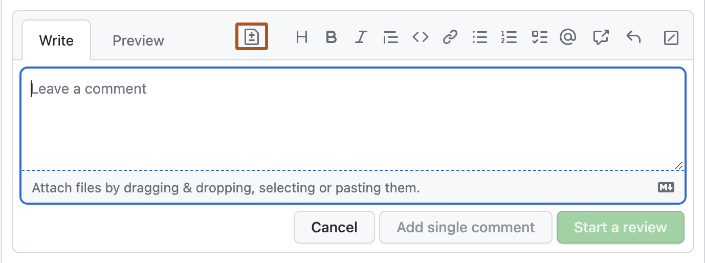
6.45.6 Ignoring Auto-Generated Files
When reviewing pull requests in R package repositories, you can typically ignore changes to .Rd files in the man/ directory. These are R documentation files automatically generated by {roxygen2} from special comments in the R source code (see Section 6.14).
Why ignore .Rd files?
- They are auto-generated and should never be manually edited
- Changes to
.Rdfiles simply reflect changes already visible in the roxygen2 comments - Reviewing the source roxygen2 comments is more informative and efficient
- The
.Rdfiles will be regenerated during the package build process
What to review instead:
Focus your review on the roxygen2 documentation comments in the actual R source files (.R files in the R/ directory). These special comments start with #' and appear immediately before function definitions. Any changes to function documentation will be visible there.
If the repository has a preview workflow (such as pkgdown for R packages or Quarto for documentation sites), you can also review the rendered documentation in the preview build. The preview workflow should automatically post a comment on the PR containing a link to a preview version of the revised documentation.
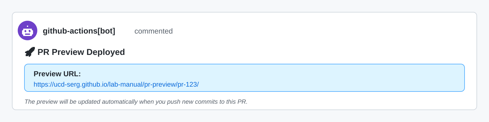
GitHub review tip:
In GitHub’s pull request “Files changed” view, you can click the three dots (...) next to a file and select “View file” to hide it from the diff view. This helps you focus on the meaningful changes.
6.45.7 Reviewing Copilot-Generated Pull Requests
When reviewing pull requests created by GitHub Copilot coding agents, apply the same standards and principles as any other PR, but be aware of some unique considerations:
Workflow approval requirements:
- You must manually approve GitHub Actions workflows for Copilot PRs
- This is a security measure because Copilot can modify any file, including workflow files themselves
- Click the approval button in the Actions tab or on the PR to trigger workflows
- There is currently no way to bypass this manual approval, even if you are the repository owner
Review focus areas:
- Verify the solution addresses the issue: Ensure Copilot understood the requirements correctly
- Check for over-engineering: Copilot may sometimes add unnecessary complexity or features beyond what was requested
- Review test coverage: Verify that tests are appropriate and comprehensive
- Check documentation: Ensure documentation is clear and follows project conventions
- Look for edge cases: AI-generated code may miss edge cases or error handling
Iterating on Copilot PRs:
When you find issues in a Copilot PR, you have two options:
Request changes from Copilot: Leave review comments and ask Copilot to address them. This works well for complex changes or when you want to see how Copilot interprets your feedback.
Make direct changes yourself: Push commits directly to the Copilot PR branch. This is often faster for simple fixes like typos, formatting, or small adjustments.
For quick fixes, you can often make changes faster than writing review comments and waiting for Copilot to respond.
Best practices:
- Don’t push while Copilot is working: Wait for Copilot to complete its current iteration before pushing your own changes to avoid merge conflicts
- Review incrementally: If a Copilot PR is large, review it in stages as the agent updates it rather than waiting until the end
- Trust but verify: Copilot is a powerful tool, but human review is essential for catching issues and ensuring quality
6.46 Creating a Pull Request Template
GitHub allows you to create a pull request template in a repository to standardize the information in pull requests. When you add a template, everyone will automatically see its contents in the pull request body.
Follow these steps to add a pull request template:
- On GitHub, navigate to the main page of the repository.
- Above the file list, click
Create new file. - Name the file
pull_request_template.md. GitHub will not recognize this as the template if it is named anything else. The file must be on the default branch.- To store the file in a hidden directory, name it
.github/pull_request_template.md.
- To store the file in a hidden directory, name it
- In the body of the new file, add your pull request template.
Here is an example pull request template:
# Description

## Summary of change

Please include a summary of the change, including any new functions added and example usage.

## Related Issues

Closes #(issue number)
Related to #(issue number)

## Testing

Describe how this change has been tested.

## Checklist

- [ ] Tests added/updated
- [ ] Documentation updated
- [ ] Code follows project style guidelines

## Who should review the pull request?

@username
6.47 Getting Help with Code
When you encounter a coding problem, creating a reprex (minimal reproducible example) is one of the most effective ways to get help—and often helps you solve the problem yourself.
A good reprex (Bryan et al. 2024):
- Is reproducible: Contains all necessary code, including
library()calls and data - Is minimal: Strips away everything not directly related to your problem
- Uses small, simple example data (often built-in datasets)
Why create a reprex:
- 80% of the time, creating a reprex helps you discover the solution yourself
- 20% of the time, you’ll have a clear example that makes it easy for others to help you
- It respects others’ time by making your problem easy to understand and reproduce
Resources:
{reprex}package: Automates creation of reproducible examples- R for Data Science: Making a reprex (Wickham et al. 2023): Step-by-step guide to creating effective reproducible examples
6.48 Additional Resources
6.48.1 R Package Development
- R Packages (Wickham and Bryan 2023) - comprehensive guide to R package development
- Tidyverse design guide (Wickham 2023) - principles for designing R packages and APIs that are intuitive, composable, and consistent with tidyverse philosophy
- usethis documentation - workflow automation for R projects
- devtools documentation - essential development tools
- pkgdown documentation - create package websites
- testthat documentation - unit testing framework
6.48.2 General R Programming
- R for Data Science (Wickham et al. 2023) - learn data science with the tidyverse
- Advanced R (Wickham 2019) - deep dive into R programming and internals
6.48.3 Shiny Development
- Mastering Shiny (Wickham 2021) - comprehensive guide to building web applications with Shiny
- Engineering Production-Grade Shiny Apps (Fay et al. 2021) - best practices for production Shiny applications
6.48.4 Git and Version Control
- Happy Git and GitHub for the useR (Bryan 2023) - essential guide to using Git and GitHub with R
{gitdown}- R package for documenting git commit history as a bookdown report, organized by patterns like tags or issues
6.14.7 Comments in the body of your code
Commenting your code is an important part of reproducibility and helps document your code for the future. When things change or break, you’ll be thankful for comments. There’s no need to comment excessively or unnecessarily, but a comment describing what a large or complex chunk of code does is always helpful. See this file for an example of how to comment your code and notice that comments are always in the form of:
See also Section 7.2 for function documentation style guidelines.