Getting Started with serodynamics • serodynamics

Introduction

The serodynamics package provides tools for modeling longitudinal antibody responses to infection using Bayesian MCMC methods. This vignette demonstrates the main workflow for:

Loading or simulating case data
Preparing data for MCMC analysis
Running the Bayesian model
Visualizing and interpreting results

Installation

First, ensure you have JAGS installed on your system (required for Bayesian MCMC):

Ubuntu/Linux: sudo apt-get install jags
macOS: Download from JAGS website
Windows: Download from JAGS website

Then install the package. This article documents the development version, so install that:

# install.packages("pak")
pak::pak("UCD-SERG/serodynamics")

A released version is also available on CRAN:

install.packages("serodynamics")

The released version uses an older set of function names, listed below for reference. Renaming calls is not enough to run this article on the released version, so install the development version as shown above.

This article	Released version
`run_serodynamics()`	`run_mod()`
`plot_trace()`	`plot_jags_trace()`
`plot_density()`	`plot_jags_dens()`
`plot_rhat()`	`plot_jags_Rhat()`
`plot_ess()`	`plot_jags_effect()`
`summarize_posterior()`	`post_summ()`

Load Required Libraries

library(serodynamics)
library(runjags)
library(dplyr)
library(ggplot2)

# Verify JAGS is installed
runjags::findJAGS()
#> [1] "/usr/bin/jags"

Example 1: Using Existing Data

The package includes example data from the SEES Typhoid study in Nepal:

data(nepal_sees)
head(nepal_sees)
#> # A tibble: 6 × 9
#>   Country id      sample_id bldculres antigen_iso studyvisit dayssincefeveronset
#>   <chr>   <chr>   <chr>     <chr>     <chr>       <chr>                    <dbl>
#> 1 Nepal   sees_n… N000_122  typhi     HlyE_IgA    28_days                     40
#> 2 Nepal   sees_n… N000_122  typhi     HlyE_IgG    28_days                     40
#> 3 Nepal   sees_n… N000_297  typhi     HlyE_IgA    3_months                   135
#> 4 Nepal   sees_n… N000_297  typhi     HlyE_IgG    3_months                   135
#> 5 Nepal   sees_n… N000_372  typhi     HlyE_IgA    6_months                   171
#> 6 Nepal   sees_n… N000_372  typhi     HlyE_IgG    6_months                   171
#> # ℹ 2 more variables: result <dbl>, visit_num <int>

Prepare the Data

Convert the data to a case_data object (nepal_sees already is a case_data object, but we can reconvert it just to demonstrate).

case_data <- as_case_data(
  nepal_sees,
  id_var = "id",
  time_in_days = "dayssincefeveronset",
  value_var = "result",
  biomarker_var = "antigen_iso"
)

# View the structure
head(case_data)
#> # A tibble: 6 × 9
#>   Country id      sample_id bldculres antigen_iso studyvisit dayssincefeveronset
#>   <chr>   <chr>   <chr>     <chr>     <chr>       <chr>                    <dbl>
#> 1 Nepal   sees_n… N000_122  typhi     HlyE_IgA    28_days                     40
#> 2 Nepal   sees_n… N000_122  typhi     HlyE_IgG    28_days                     40
#> 3 Nepal   sees_n… N000_297  typhi     HlyE_IgA    3_months                   135
#> 4 Nepal   sees_n… N000_297  typhi     HlyE_IgG    3_months                   135
#> 5 Nepal   sees_n… N000_372  typhi     HlyE_IgA    6_months                   171
#> 6 Nepal   sees_n… N000_372  typhi     HlyE_IgG    6_months                   171
#> # ℹ 2 more variables: result <dbl>, visit_num <int>

Visualize the Raw Data

autoplot(case_data)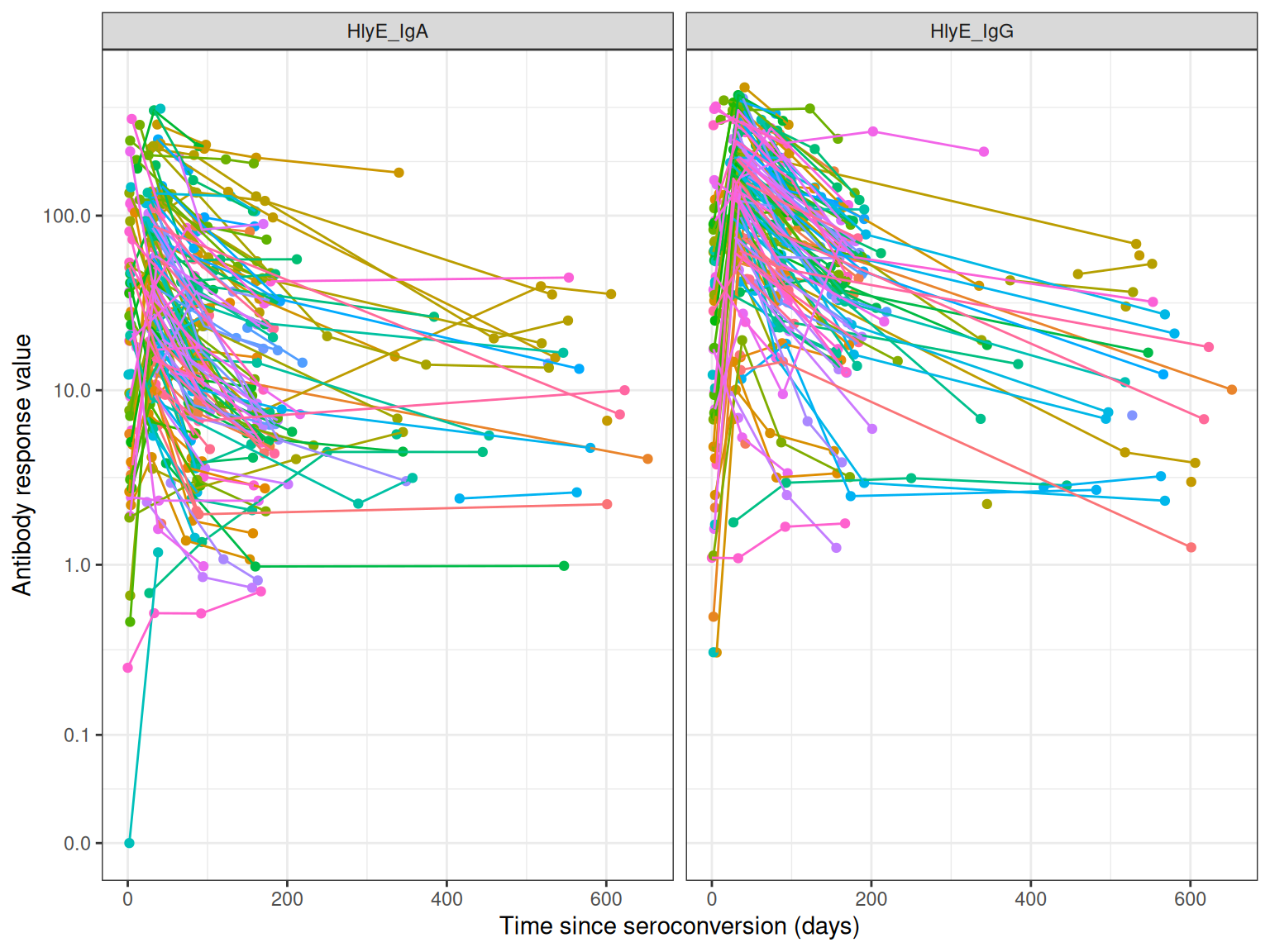

Example 2: Simulating Data

You can also simulate case data using antibody curve parameters:

set.seed(123)

# Use typhoid curve parameters from serocalculator
simulated_data <- sim_case_data(
  n = 50,  # Number of cases to simulate
  curve_params = serocalculator::typhoid_curves_nostrat_100,
  max_n_obs = 6,  # Maximum observations per case
  followup_interval = 14  # Days between follow-up visits
)

head(simulated_data)
#> # A tibble: 6 × 11
#>   id    visit_num timeindays  iter antigen_iso    y0     y1    t1    alpha     r
#>   <chr>     <int>      <dbl> <int> <fct>       <dbl>  <dbl> <dbl>    <dbl> <dbl>
#> 1 1             1          0    89 HlyE_IgA    0.666   47.1  7.18  5.22e-4  1.56
#> 2 1             1          0    89 HlyE_IgG    3.52   266.   5.60  1.25e-3  1.53
#> 3 1             1          0    89 LPS_IgA     1.77  2071.   1.71  2.21e-5  3.45
#> 4 1             1          0    89 LPS_IgG     0.200  234.   5.30  1.69e-3  1.28
#> 5 1             1          0    89 Vi_IgG      1.66   543.   8.37  3.72e-5  1.26
#> 6 1             2         14    89 HlyE_IgA    0.666   47.1  7.18  5.22e-4  1.56
#> # ℹ 1 more variable: value <dbl>

autoplot(simulated_data)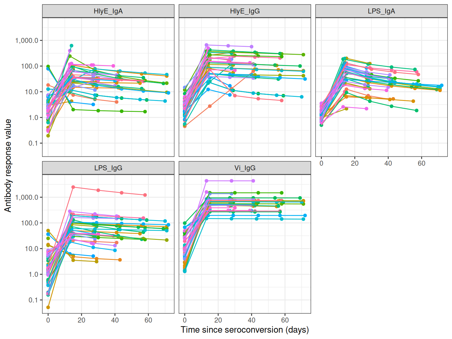

Running the Bayesian Model

The main function run_serodynamics() fits a Bayesian MCMC model to estimate antibody dynamic curve parameters:

y0: Baseline antibody concentration
y1: Peak antibody concentration
t1: Time to peak
shape: Shape parameter
alpha: Decay rate

# Note: This example uses reduced iterations for demonstration
# For actual analysis, use larger values (e.g., nmc=1000, niter=2000)

fitted_model <- run_serodynamics(
  data = simulated_data,
  file_mod = serodynamics_example("model.jags"),
  nchain = 2,      # Number of MCMC chains
  nadapt = 100,    # Adaptation iterations
  nburn = 100,     # Burn-in iterations  
  nmc = 10,        # Samples per chain (use 1000+ for real analysis)
  niter = 20       # Total iterations (use 2000+ for real analysis)
)
#> Calling 2 simulations using the parallel method...
#> Following the progress of chain 1 (the program will wait for all chains
#> to finish before continuing):
#> Welcome to JAGS 4.3.2 on Wed Sep  2 21:23:31 2026
#> JAGS is free software and comes with ABSOLUTELY NO WARRANTY
#> Loading module: basemod: ok
#> Loading module: bugs: ok
#> . . Reading data file data.txt
#> . Compiling model graph
#>    Resolving undeclared variables
#>    Allocating nodes
#> Graph information:
#>    Observed stochastic nodes: 815
#>    Unobserved stochastic nodes: 285
#>    Total graph size: 14771
#> . Reading parameter file inits1.txt
#> . Initializing model
#> . Adapting 100
#> -------------------------------------------------| 100
#> ++++++++++++++++++++++++++++++++++++++++++++++++++ 100%
#> Adaptation incomplete.
#> . Updating 100
#> -------------------------------------------------| 100
#> ************************************************** 100%
#> . . . . . . Updating 20
#> . . . . Updating 0
#> . Deleting model
#> . 
#> All chains have finished
#> Warning: The adaptation phase of one or more models was not completed in 100
#> iterations, so the current samples may not be optimal - try increasing the
#> number of iterations to the "adapt" argument
#> Simulation complete.  Reading coda files...
#> Coda files loaded successfully
#> Finished running the simulation

head(fitted_model)
#> # A tibble: 6 × 7
#>   Iteration Chain Parameter Iso_type Stratification Subject  value
#>       <int> <int> <chr>     <chr>    <chr>          <chr>    <dbl>
#> 1         1     1 alpha     HlyE_IgA None           1       0.0114
#> 2         2     1 alpha     HlyE_IgA None           1       0.0114
#> 3         3     1 alpha     HlyE_IgA None           1       0.0114
#> 4         4     1 alpha     HlyE_IgA None           1       0.0114
#> 5         5     1 alpha     HlyE_IgA None           1       0.0217
#> 6         6     1 alpha     HlyE_IgA None           1       0.0217

Model Diagnostics

After fitting the model, check convergence diagnostics:

# Trace plots to assess chain mixing
plot_trace(fitted_model)
#> $None
#> $None$HlyE_IgA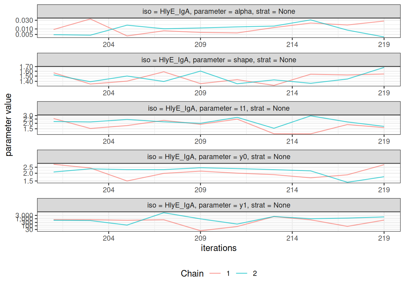

#>
#> $None$HlyE_IgG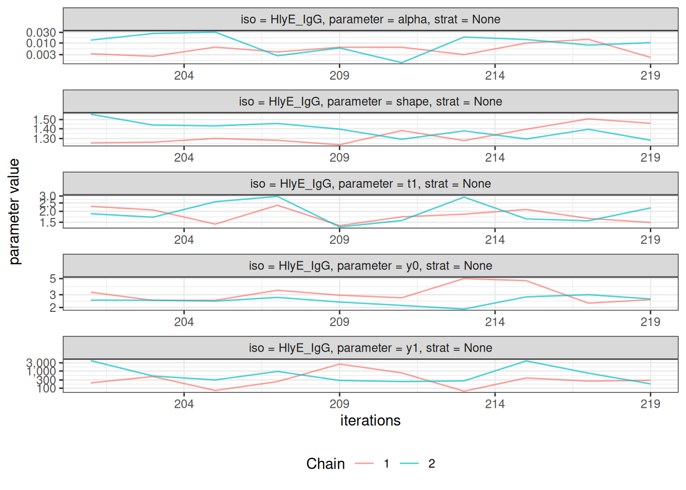

#>
#> $None$LPS_IgA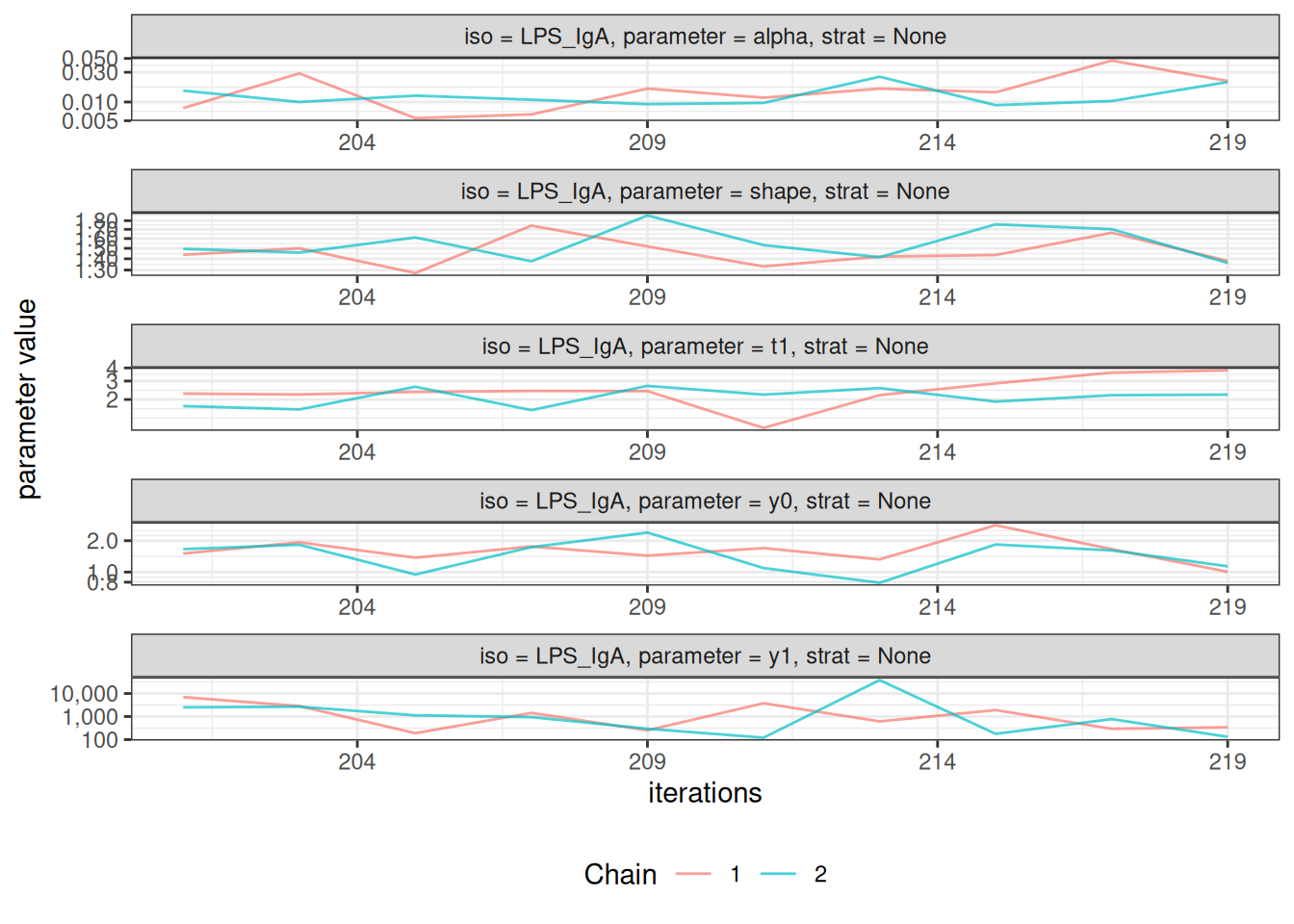

#>
#> $None$LPS_IgG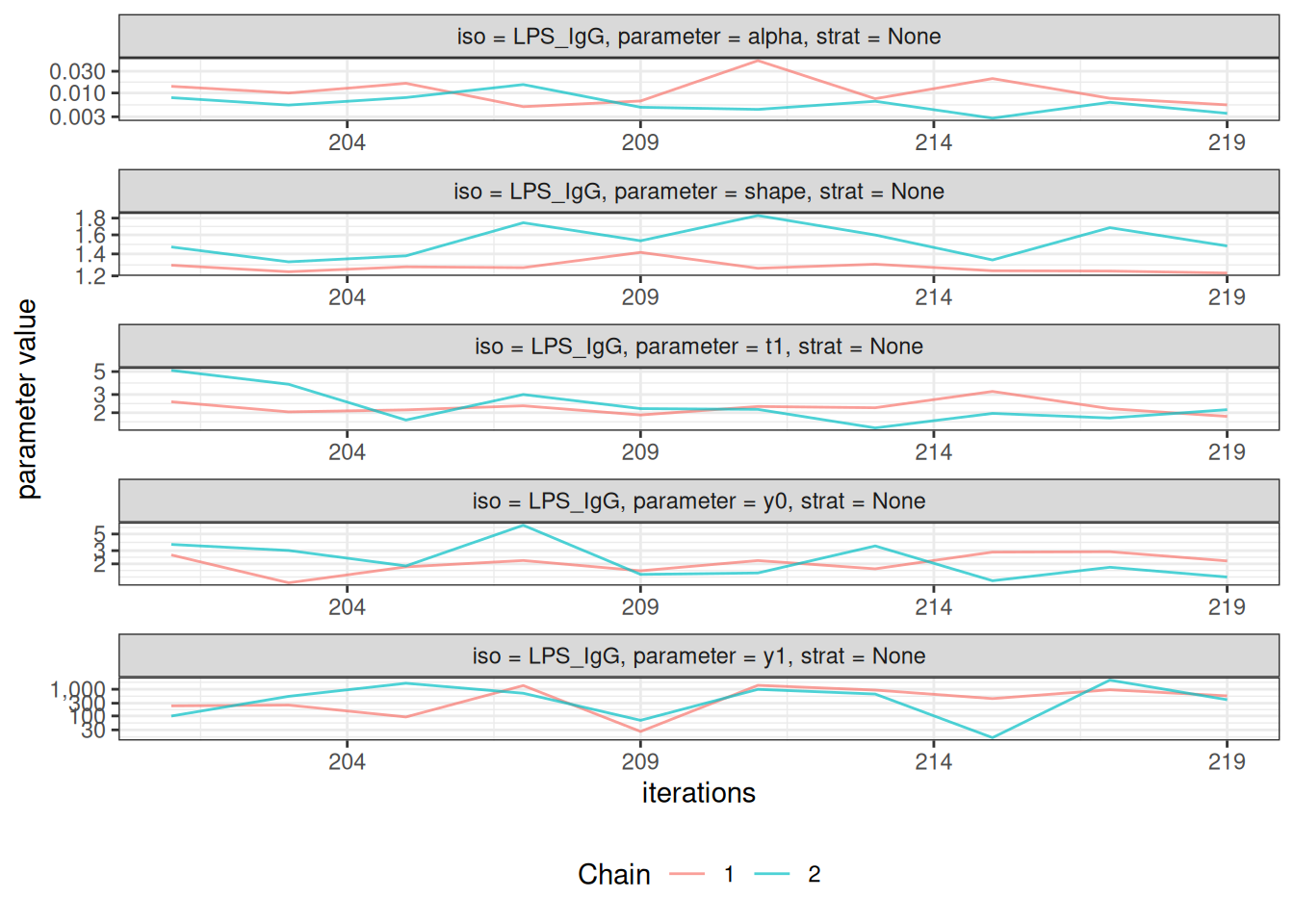

#>
#> $None$Vi_IgG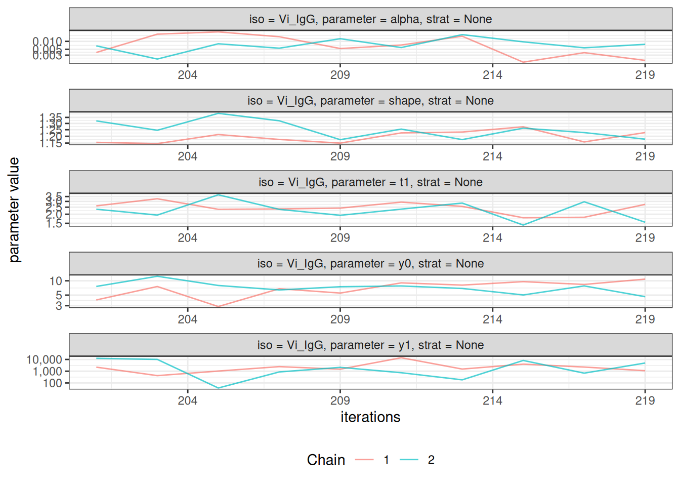


# Density plots of posterior distributions
plot_density(fitted_model)
#> $None
#> $None$HlyE_IgA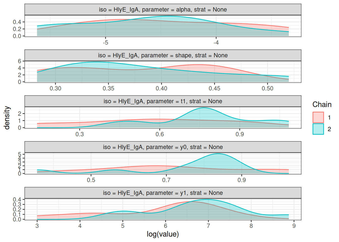

#>
#> $None$HlyE_IgG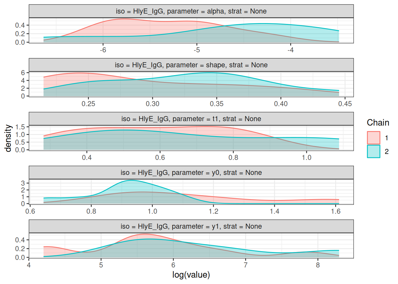

#>
#> $None$LPS_IgA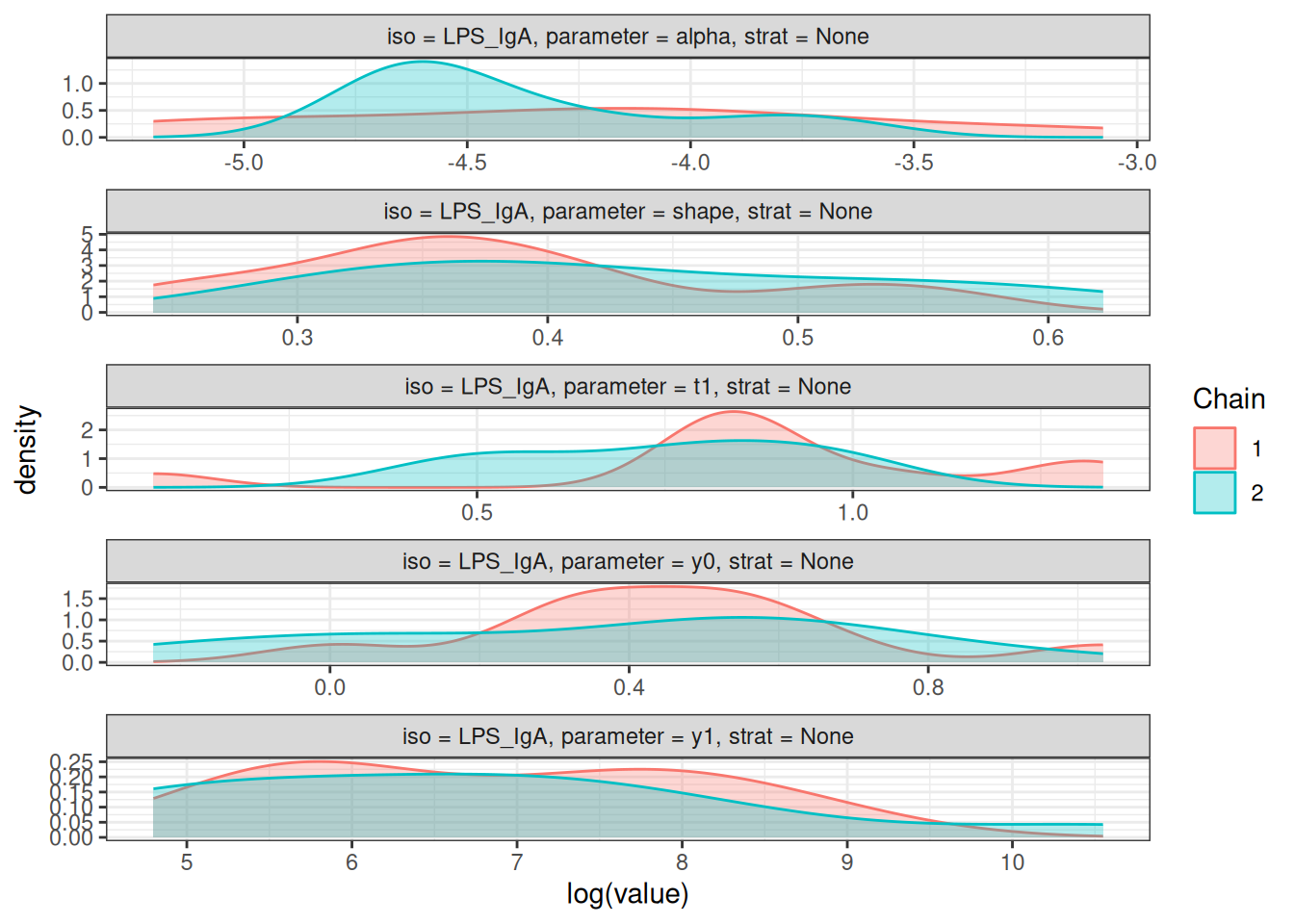

#>
#> $None$LPS_IgG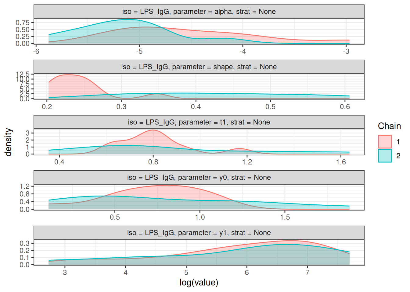

#>
#> $None$Vi_IgG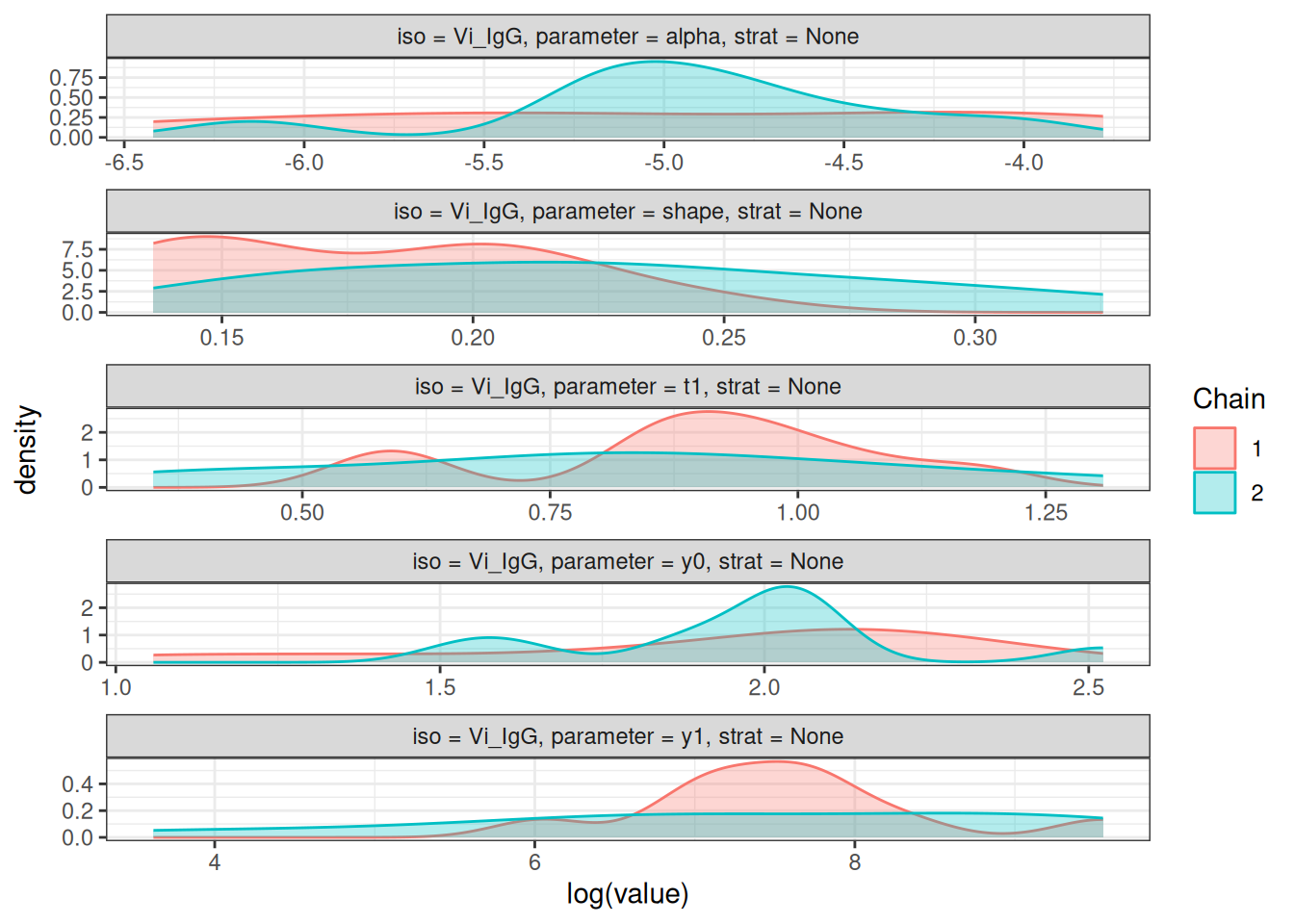


# Rhat statistics (values near 1.0 indicate convergence)
plot_rhat(fitted_model)
#> $None
#> $None$HlyE_IgA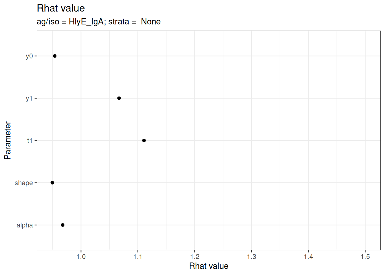

#>
#> $None$HlyE_IgG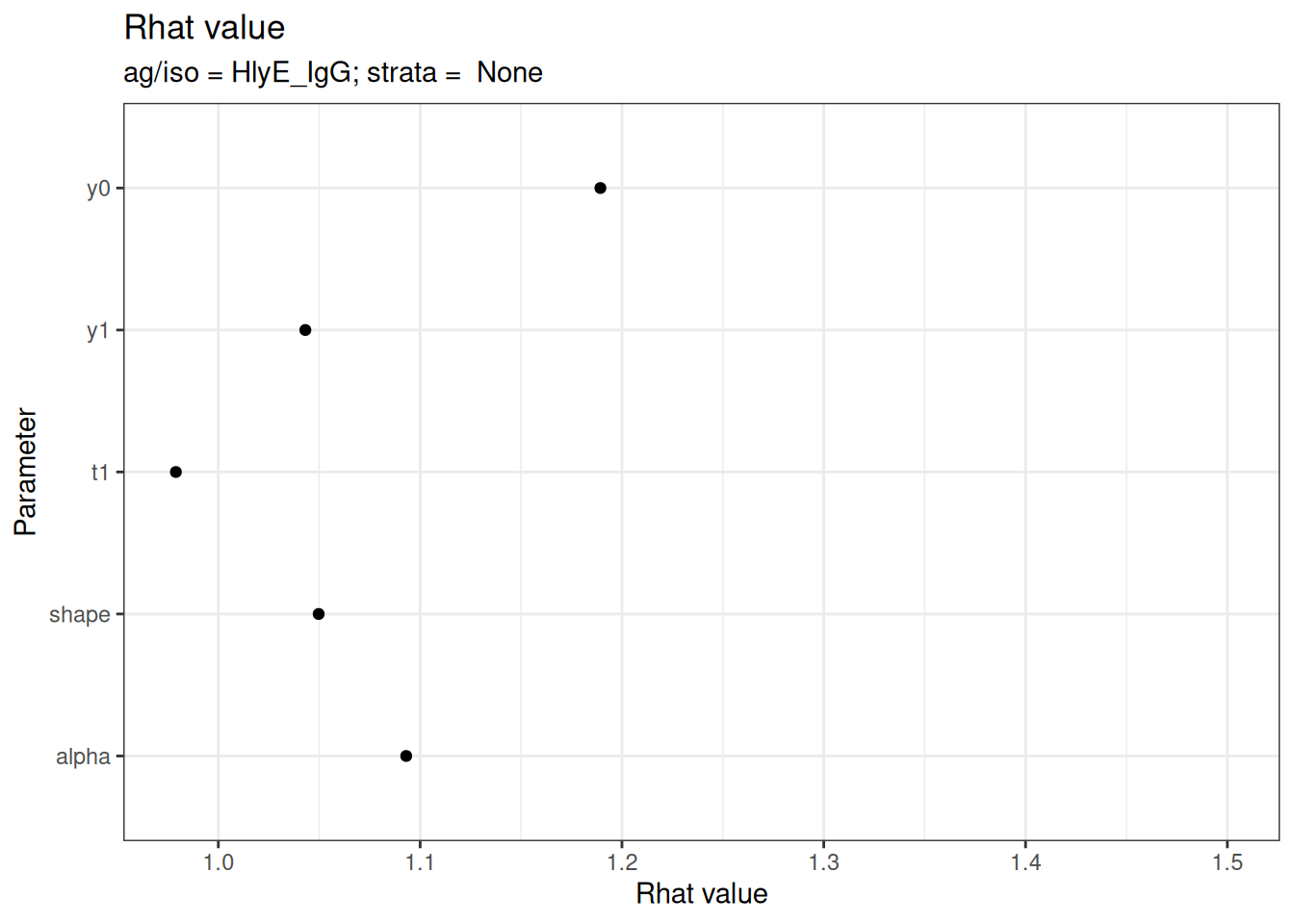

#>
#> $None$LPS_IgA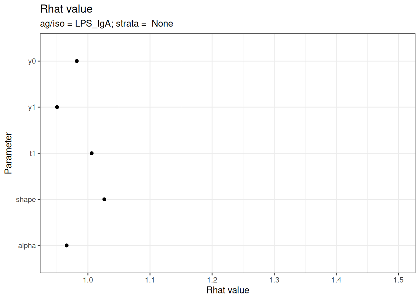

#>
#> $None$LPS_IgG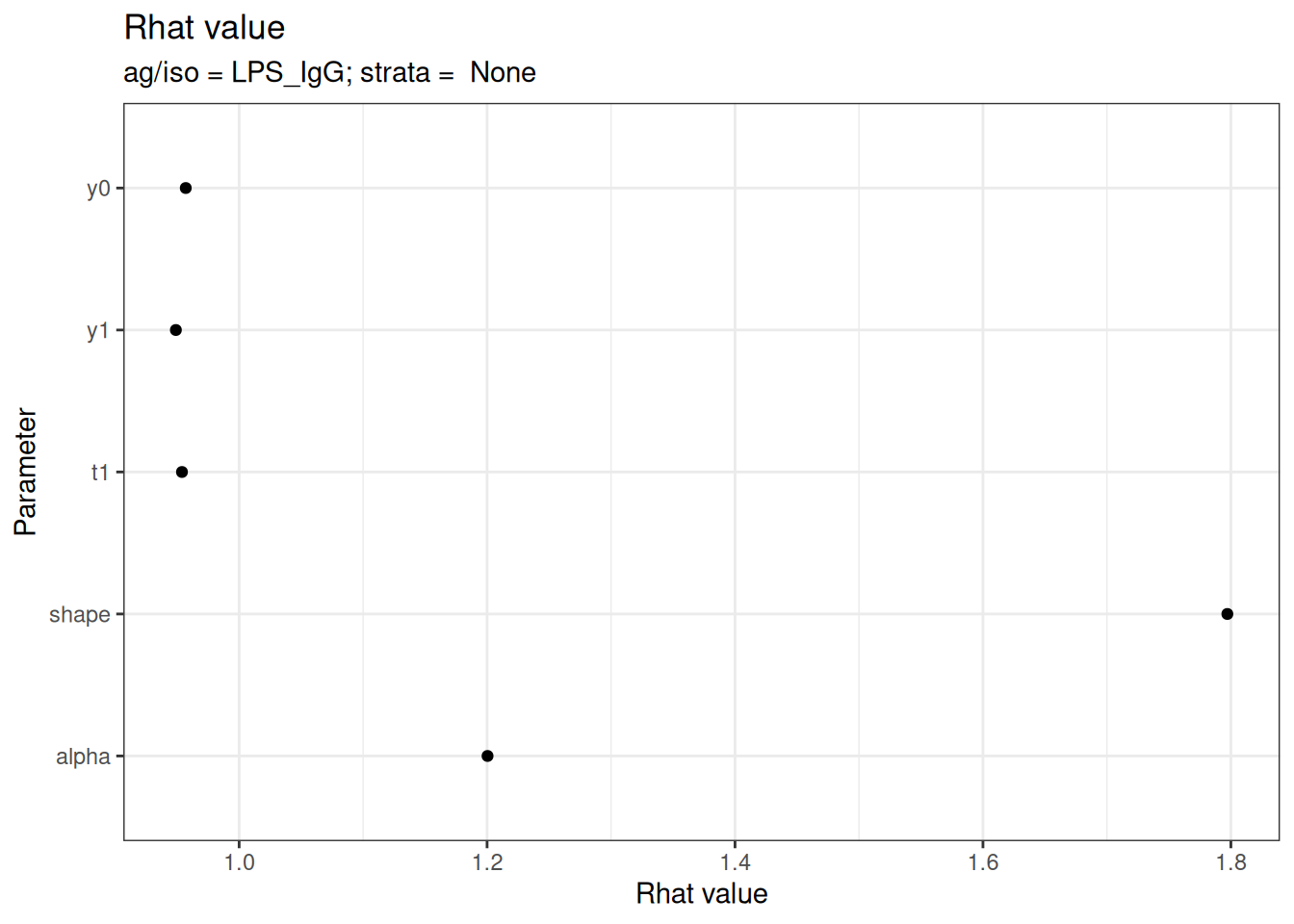

#>
#> $None$Vi_IgG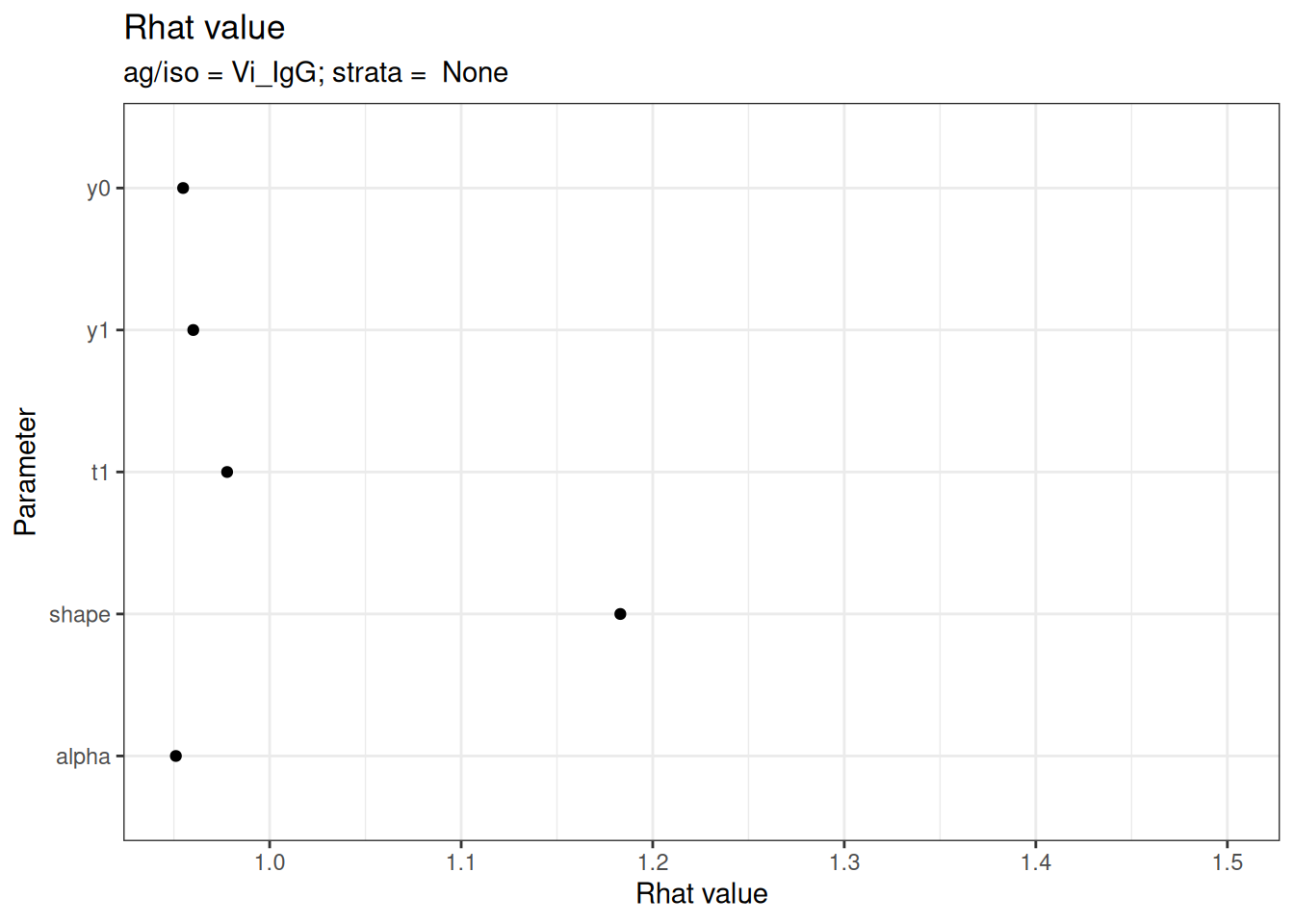


# Effective sample size
plot_ess(fitted_model)
#> $None
#> $None$HlyE_IgA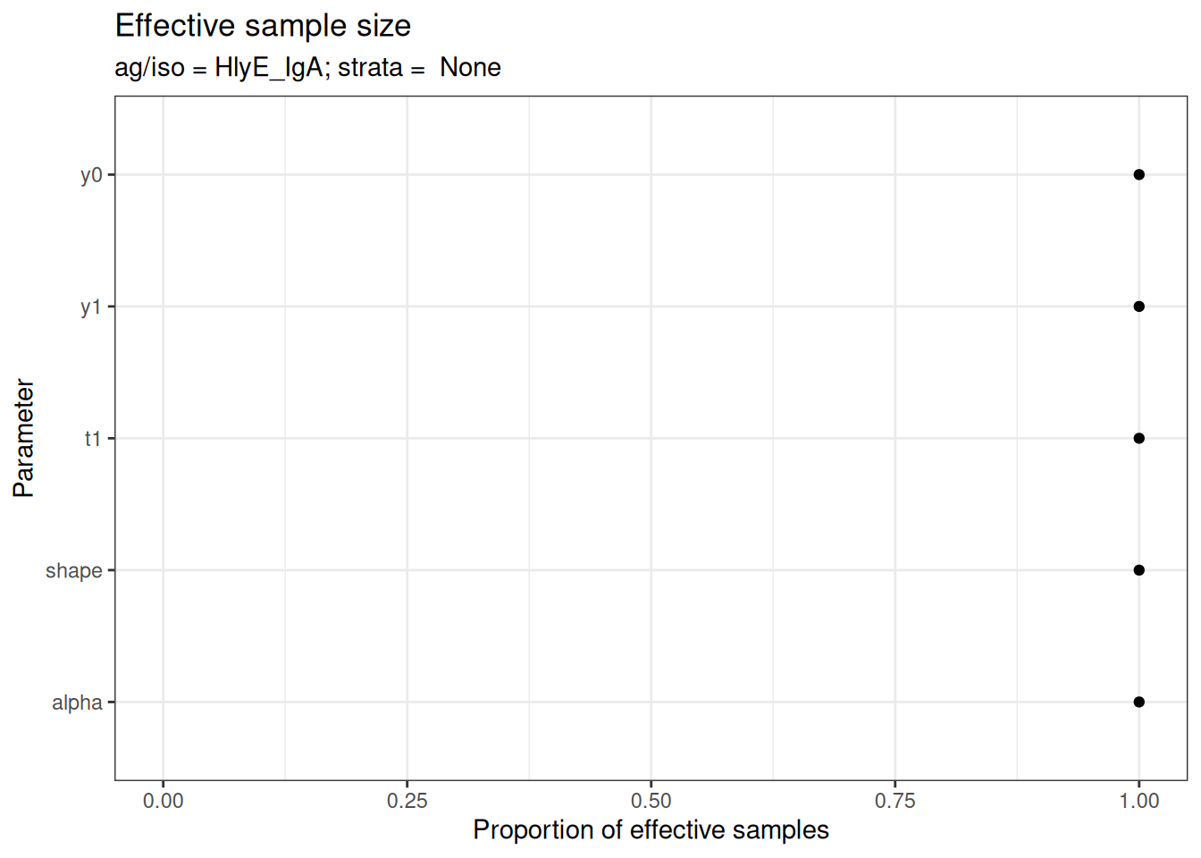

#>
#> $None$HlyE_IgG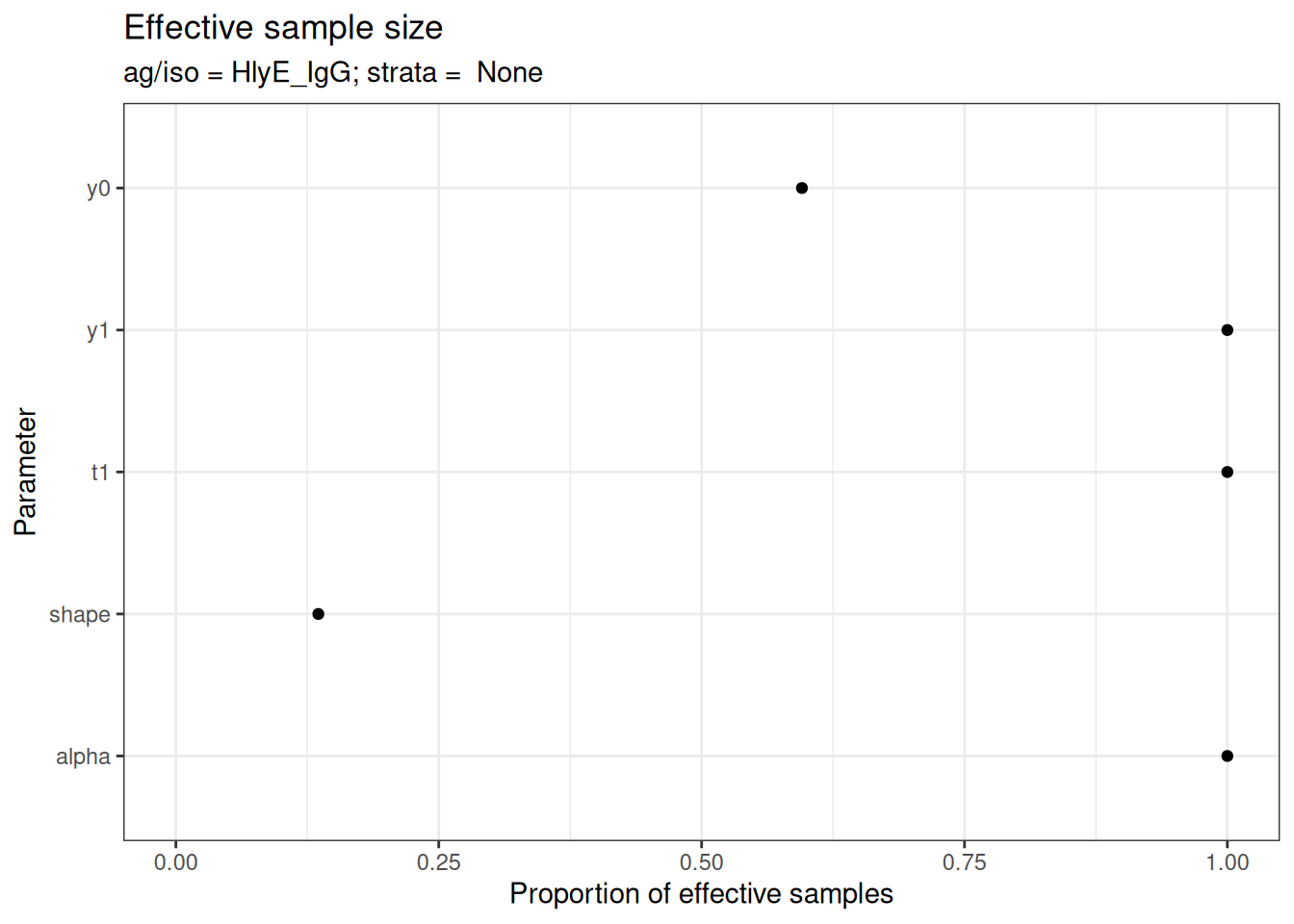

#>
#> $None$LPS_IgA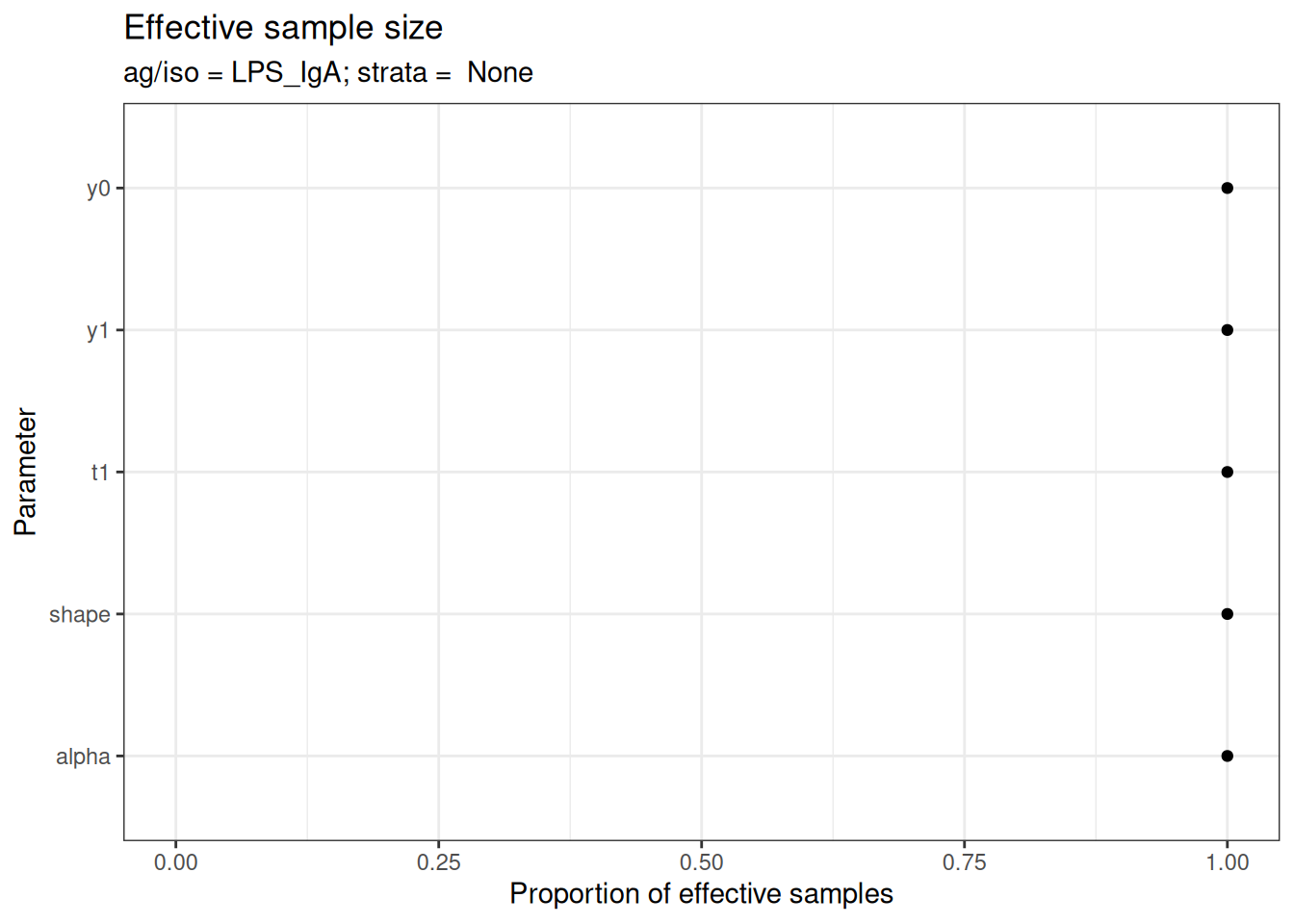

#>
#> $None$LPS_IgG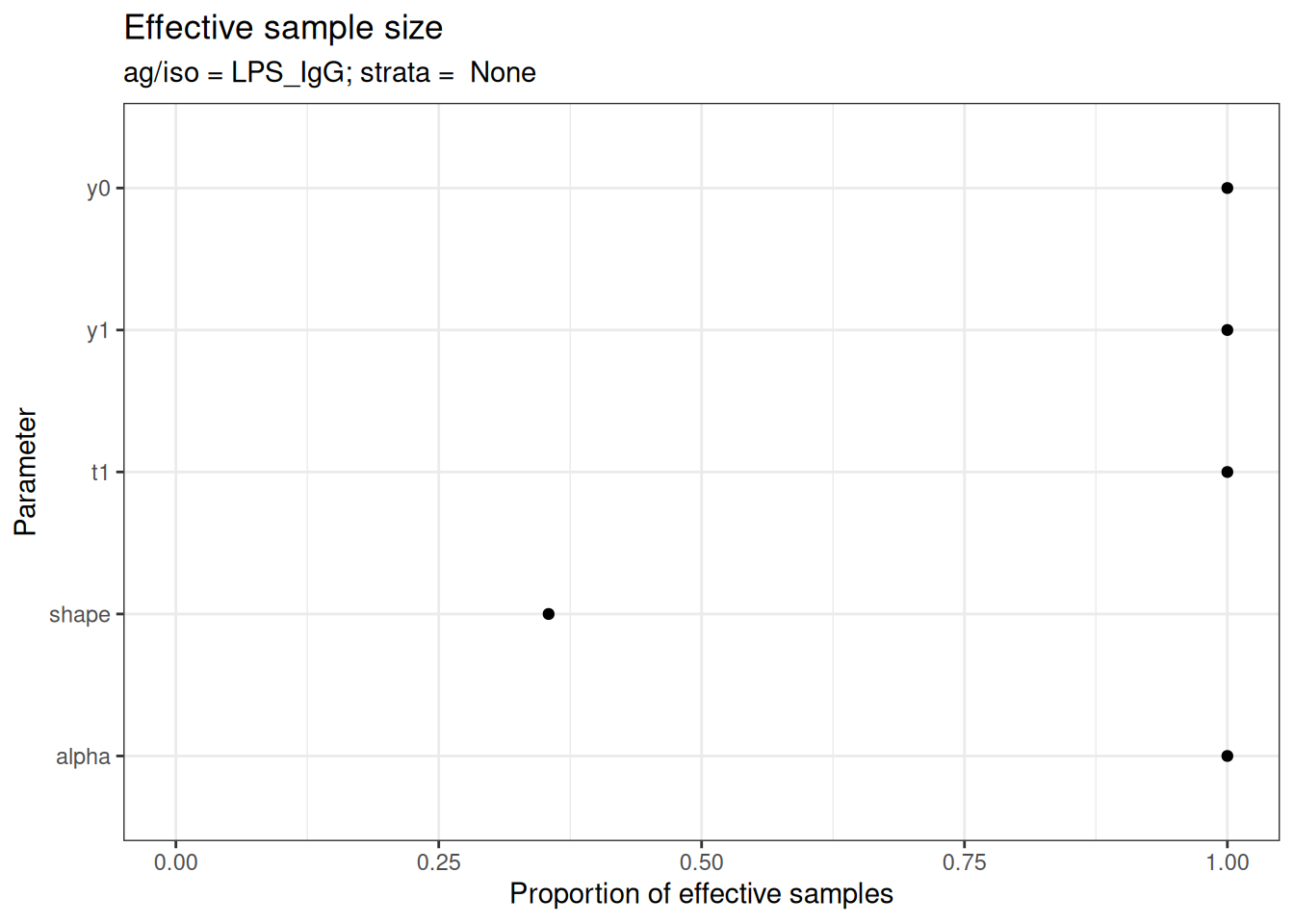

#>
#> $None$Vi_IgG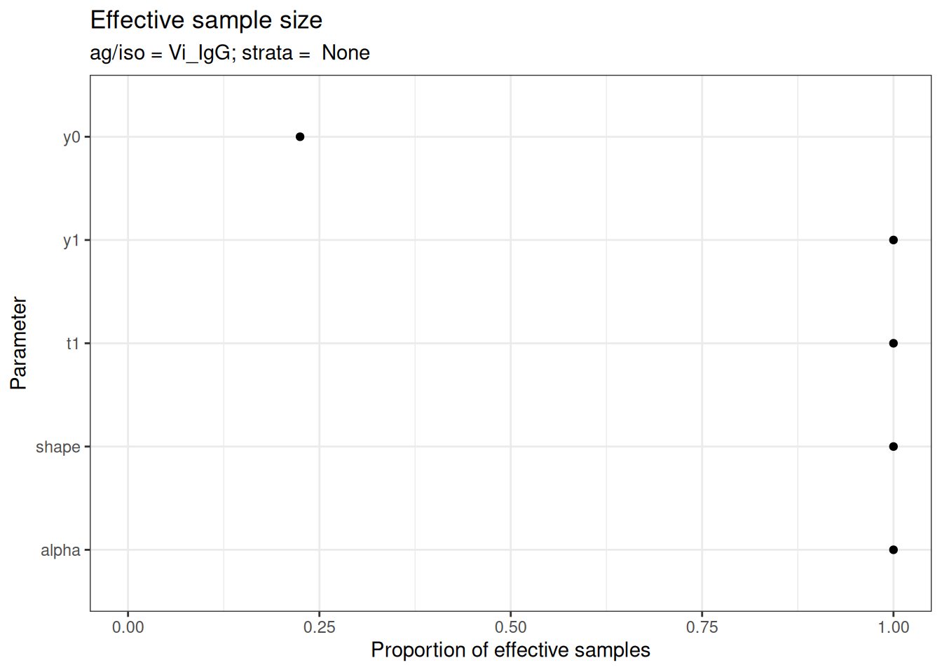

Visualizing Fitted Curves

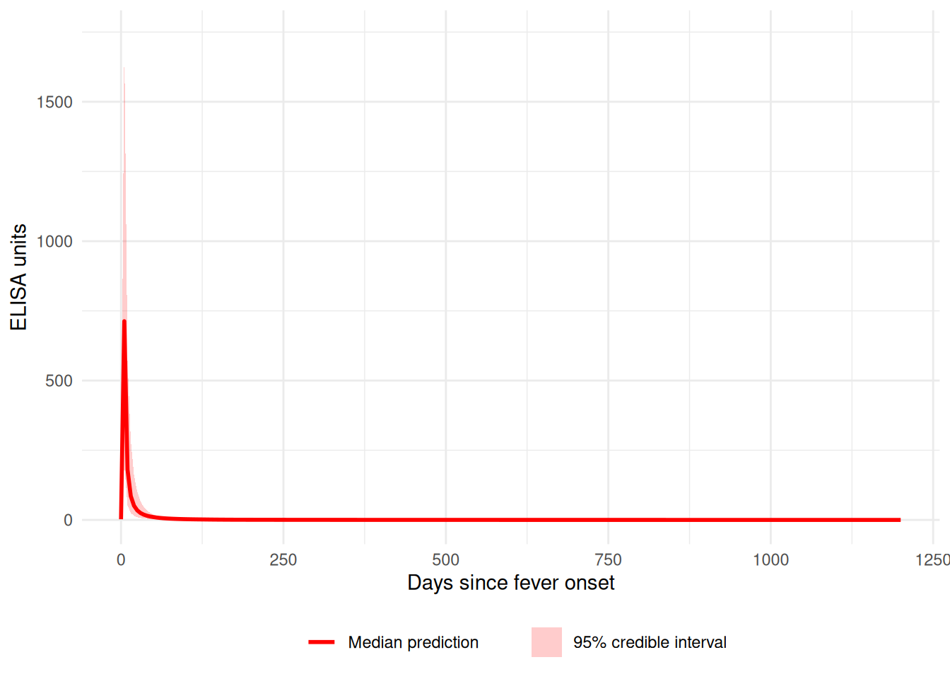
Plot the predicted antibody curves with credible intervals:

plot_predicted_curve(
  fitted_model,
  ids = serocalculator::ids(simulated_data)[1],
  antigen_iso = simulated_data$antigen_iso[1]
)

Post-Processing Results

Extract and summarize the posterior estimates:

# Summarize parameter estimates
summary_stats <- summarize_posterior(fitted_model)
print(summary_stats)
#> # A tibble: 25 × 11
#>    Iso_type Parameter Stratification       Mean       SD  Median  `2.5%` `25.0%`
#>    <chr>    <chr>     <chr>               <dbl>    <dbl>   <dbl>   <dbl>   <dbl>
#>  1 HlyE_IgA alpha     None              0.0132   9.15e-3 1.08e-2 3.87e-3 6.37e-3
#>  2 HlyE_IgA shape     None              1.47     1.01e-1 1.44e+0 1.34e+0 1.39e+0
#>  3 HlyE_IgA t1        None              2.02     4.93e-1 2.07e+0 1.15e+0 1.67e+0
#>  4 HlyE_IgA y0        None              2.13     3.68e-1 2.17e+0 1.46e+0 1.89e+0
#>  5 HlyE_IgA y1        None           1105.       1.55e+3 7.14e+2 4.82e+1 4.59e+2
#>  6 HlyE_IgG alpha     None              0.00956  8.14e-3 6.50e-3 1.77e-3 3.22e-3
#>  7 HlyE_IgG shape     None              1.36     9.20e-2 1.38e+0 1.25e+0 1.28e+0
#>  8 HlyE_IgG t1        None              1.94     4.89e-1 1.80e+0 1.35e+0 1.57e+0
#>  9 HlyE_IgG y0        None              2.85     7.70e-1 2.60e+0 2.01e+0 2.49e+0
#> 10 HlyE_IgG y1        None            833.       1.19e+3 2.95e+2 7.01e+1 2.42e+2
#> # ℹ 15 more rows
#> # ℹ 3 more variables: `50.0%` <dbl>, `75.0%` <dbl>, `97.5%` <dbl>

Working with Stratified Data

You can stratify the analysis by a grouping variable:

# Create stratified data
strat1 <- sim_case_data(
  n = 30, 
  curve_params = serocalculator::typhoid_curves_nostrat_100
) |>
  mutate(pathogen = "Typhoid")

strat2 <- sim_case_data(
  n = 30,
  curve_params = serocalculator::typhoid_curves_nostrat_100  
) |>
  mutate(pathogen = "Paratyphoid")

stratified_data <- bind_rows(strat1, strat2)

# Fit model with stratification
fitted_stratified <- run_serodynamics(
  data = stratified_data,
  file_mod = serodynamics_example("model.jags"),
  nchain = 2,
  nadapt = 100,
  nburn = 100,
  nmc = 10,
  niter = 20,
  strat = "pathogen"  # Specify stratification variable
)
#> Calling 2 simulations using the parallel method...
#> Following the progress of chain 1 (the program will wait for all chains
#> to finish before continuing):
#> Welcome to JAGS 4.3.2 on Wed Sep  2 21:23:41 2026
#> JAGS is free software and comes with ABSOLUTELY NO WARRANTY
#> Loading module: basemod: ok
#> Loading module: bugs: ok
#> . . Reading data file data.txt
#> . Compiling model graph
#>    Resolving undeclared variables
#>    Allocating nodes
#> Graph information:
#>    Observed stochastic nodes: 775
#>    Unobserved stochastic nodes: 185
#>    Total graph size: 12303
#> . Reading parameter file inits1.txt
#> . Initializing model
#> . Adapting 100
#> -------------------------------------------------| 100
#> ++++++++++++++++++++++++++++++++++++++++++++++++++ 100%
#> Adaptation incomplete.
#> . Updating 100
#> -------------------------------------------------| 100
#> ************************************************** 100%
#> . . . . . . Updating 20
#> . . . . Updating 0
#> . Deleting model
#> . 
#> All chains have finished
#> Warning: The adaptation phase of one or more models was not completed in 100
#> iterations, so the current samples may not be optimal - try increasing the
#> number of iterations to the "adapt" argument
#> Simulation complete.  Reading coda files...
#> Coda files loaded successfully
#> Finished running the simulation
#> Calling 2 simulations using the parallel method...
#> Following the progress of chain 1 (the program will wait for all chains
#> to finish before continuing):
#> Welcome to JAGS 4.3.2 on Wed Sep  2 21:23:43 2026
#> JAGS is free software and comes with ABSOLUTELY NO WARRANTY
#> Loading module: basemod: ok
#> Loading module: bugs: ok
#> . . Reading data file data.txt
#> . Compiling model graph
#>    Resolving undeclared variables
#>    Allocating nodes
#> Graph information:
#>    Observed stochastic nodes: 760
#>    Unobserved stochastic nodes: 185
#>    Total graph size: 12135
#> . Reading parameter file inits1.txt
#> . Initializing model
#> . Adapting 100
#> -------------------------------------------------| 100
#> ++++++++++++++++++++++++++++++++++++++++++++++++++ 100%
#> Adaptation incomplete.
#> . Updating 100
#> -------------------------------------------------| 100
#> ************************************************** 100%
#> . . . . . . Updating 20
#> . . . . Updating 0
#> . Deleting model
#> . 
#> All chains have finished
#> Warning: The adaptation phase of one or more models was not completed in 100
#> iterations, so the current samples may not be optimal - try increasing the
#> number of iterations to the "adapt" argument
#> Simulation complete.  Reading coda files...
#> Coda files loaded successfully
#> Finished running the simulation

Next Steps

See the function reference for complete API documentation
Check out example datasets: ?nepal_sees, ?nepal_sees_jags_output

Session Info

sessioninfo::session_info()
#> ─ Session info ───────────────────────────────────────────────────────────────
#>  setting  value
#>  version  R version 4.6.1 (2026-06-24)
#>  os       Ubuntu 24.04.4 LTS
#>  system   x86_64, linux-gnu
#>  ui       X11
#>  language en-US
#>  collate  C.UTF-8
#>  ctype    C.UTF-8
#>  tz       UTC
#>  date     2026-09-02
#>  pandoc   3.8.3 @ /opt/hostedtoolcache/pandoc/3.8.3/x64/ (via rmarkdown)
#>  quarto   1.10.18 @ /usr/local/bin/quarto
#> 
#> ─ Packages ───────────────────────────────────────────────────────────────────
#>  package        * version    date (UTC) lib source
#>  cli              3.6.6      2026-04-09 [1] CRAN (R 4.6.1)
#>  coda             0.19-4.1   2024-01-31 [1] CRAN (R 4.6.1)
#>  codetools        0.2-20     2024-03-31 [3] CRAN (R 4.6.1)
#>  digest           0.6.39     2025-11-19 [1] CRAN (R 4.6.1)
#>  doParallel       1.0.17     2022-02-07 [1] CRAN (R 4.6.1)
#>  dplyr          * 1.2.1      2026-04-03 [1] CRAN (R 4.6.1)
#>  evaluate         1.0.5      2025-08-27 [1] CRAN (R 4.6.1)
#>  farver           2.1.2      2024-05-13 [1] CRAN (R 4.6.1)
#>  fastmap          1.2.0      2024-05-15 [1] CRAN (R 4.6.1)
#>  foreach          1.5.2      2022-02-02 [1] CRAN (R 4.6.1)
#>  fs               2.1.0      2026-04-18 [1] CRAN (R 4.6.1)
#>  generics         0.1.4      2025-05-09 [1] CRAN (R 4.6.1)
#>  GGally           2.4.0      2025-08-23 [1] CRAN (R 4.6.1)
#>  ggmcmc           1.5.1.2    2025-10-02 [1] CRAN (R 4.6.1)
#>  ggplot2        * 4.0.3      2026-04-22 [1] CRAN (R 4.6.1)
#>  ggstats          0.14.0     2026-09-02 [1] CRAN (R 4.6.1)
#>  glue             1.8.1      2026-04-17 [1] CRAN (R 4.6.1)
#>  gtable           0.3.6      2024-10-25 [1] CRAN (R 4.6.1)
#>  htmltools        0.5.9      2025-12-04 [1] CRAN (R 4.6.1)
#>  iterators        1.0.14     2022-02-05 [1] CRAN (R 4.6.1)
#>  jsonlite         2.0.0      2025-03-27 [1] CRAN (R 4.6.1)
#>  knitr            1.51       2025-12-20 [1] CRAN (R 4.6.1)
#>  labeling         0.4.3      2023-08-29 [1] CRAN (R 4.6.1)
#>  lattice          0.22-9     2026-02-09 [3] CRAN (R 4.6.1)
#>  lifecycle        1.0.5      2026-01-08 [1] CRAN (R 4.6.1)
#>  magrittr         2.0.5      2026-04-04 [1] CRAN (R 4.6.1)
#>  MASS             7.3-65     2025-02-28 [3] CRAN (R 4.6.1)
#>  otel             0.2.0      2025-08-29 [1] CRAN (R 4.6.1)
#>  pillar           1.11.1     2025-09-17 [1] CRAN (R 4.6.1)
#>  pkgconfig        2.0.3      2019-09-22 [1] CRAN (R 4.6.1)
#>  purrr            1.2.2      2026-04-10 [1] CRAN (R 4.6.1)
#>  R6               2.6.1      2025-02-15 [1] CRAN (R 4.6.1)
#>  RColorBrewer     1.1-3      2022-04-03 [1] CRAN (R 4.6.1)
#>  Rcpp             1.1.2      2026-07-05 [1] CRAN (R 4.6.1)
#>  rlang            1.3.0      2026-07-05 [1] CRAN (R 4.6.1)
#>  rmarkdown        2.32       2026-09-01 [1] CRAN (R 4.6.1)
#>  rngtools         1.5.2      2021-09-20 [1] CRAN (R 4.6.1)
#>  runjags        * 2.2.2-5    2025-04-09 [1] CRAN (R 4.6.1)
#>  S7               0.2.2      2026-04-22 [1] CRAN (R 4.6.1)
#>  scales           1.4.0      2025-04-24 [1] CRAN (R 4.6.1)
#>  serocalculator   1.4.1      2026-03-25 [1] CRAN (R 4.6.1)
#>  serodynamics   * 0.1.0.9021 2026-09-02 [1] local
#>  sessioninfo      1.2.4      2026-06-04 [1] CRAN (R 4.6.1)
#>  tibble           3.3.1      2026-01-11 [1] CRAN (R 4.6.1)
#>  tidyr            1.3.2      2025-12-19 [1] CRAN (R 4.6.1)
#>  tidyselect       1.2.1      2024-03-11 [1] CRAN (R 4.6.1)
#>  utf8             1.2.6      2025-06-08 [1] CRAN (R 4.6.1)
#>  vctrs            0.7.3      2026-04-11 [1] CRAN (R 4.6.1)
#>  withr            3.0.3      2026-06-19 [1] CRAN (R 4.6.1)
#>  xfun             0.60       2026-07-09 [1] CRAN (R 4.6.1)
#>  yaml             2.3.12     2025-12-10 [1] CRAN (R 4.6.1)
#> 
#>  [1] /home/runner/work/_temp/Library
#>  [2] /opt/R/4.6.1/lib/R/site-library
#>  [3] /opt/R/4.6.1/lib/R/library
#>  * ── Packages attached to the search path.
#> 
#> ──────────────────────────────────────────────────────────────────────────────