Getting Started with serodynamics

Introduction

The serodynamics package provides tools for modeling longitudinal antibody responses to infection using Bayesian MCMC methods. This vignette demonstrates the main workflow for:

1. Loading or simulating case data
2. Preparing data for MCMC analysis
3. Running the Bayesian model
4. Visualizing and interpreting results

Installation

First, ensure you have JAGS installed on your system (required for Bayesian MCMC):

• Ubuntu/Linux: sudo apt-get install jags
• macOS: Download from JAGS website
• Windows: Download from JAGS website

Then install the package:

# install.packages("pak")
pak::pak("UCD-SERG/serodynamics")

Load Required Libraries

library(serodynamics)
library(runjags)
library(dplyr)
library(ggplot2)

# Verify JAGS is installed
runjags::findJAGS()
#> [1] "/usr/bin/jags"

Example 1: Using Existing Data

The package includes example data from the SEES Typhoid study in Nepal:

data(nepal_sees)
head(nepal_sees)
#> # A tibble: 6 × 9
#>   Country id      sample_id bldculres antigen_iso studyvisit dayssincefeveronset
#>   <chr>   <chr>   <chr>     <chr>     <chr>       <chr>                    <dbl>
#> 1 Nepal   sees_n… N000_122  typhi     HlyE_IgA    28_days                     40
#> 2 Nepal   sees_n… N000_122  typhi     HlyE_IgG    28_days                     40
#> 3 Nepal   sees_n… N000_297  typhi     HlyE_IgA    3_months                   135
#> 4 Nepal   sees_n… N000_297  typhi     HlyE_IgG    3_months                   135
#> 5 Nepal   sees_n… N000_372  typhi     HlyE_IgA    6_months                   171
#> 6 Nepal   sees_n… N000_372  typhi     HlyE_IgG    6_months                   171
#> # ℹ 2 more variables: result <dbl>, visit_num <int>

Prepare the Data

Convert the data to a case_data object (nepal_sees already is a case_data object, but we can reconvert it just to demonstrate).

case_data <- as_case_data(
  nepal_sees,
  id_var = "id",
  time_in_days = "dayssincefeveronset",
  value_var = "result",
  biomarker_var = "antigen_iso"
)

# View the structure
head(case_data)
#> # A tibble: 6 × 9
#>   Country id      sample_id bldculres antigen_iso studyvisit dayssincefeveronset
#>   <chr>   <chr>   <chr>     <chr>     <chr>       <chr>                    <dbl>
#> 1 Nepal   sees_n… N000_122  typhi     HlyE_IgA    28_days                     40
#> 2 Nepal   sees_n… N000_122  typhi     HlyE_IgG    28_days                     40
#> 3 Nepal   sees_n… N000_297  typhi     HlyE_IgA    3_months                   135
#> 4 Nepal   sees_n… N000_297  typhi     HlyE_IgG    3_months                   135
#> 5 Nepal   sees_n… N000_372  typhi     HlyE_IgA    6_months                   171
#> 6 Nepal   sees_n… N000_372  typhi     HlyE_IgG    6_months                   171
#> # ℹ 2 more variables: result <dbl>, visit_num <int>

Visualize the Raw Data

autoplot(case_data)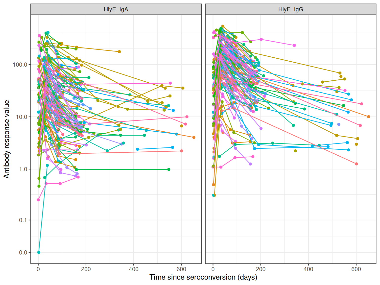

Example 2: Simulating Data

You can also simulate case data using antibody curve parameters:

set.seed(123)

# Use typhoid curve parameters from serocalculator
simulated_data <- sim_case_data(
  n = 50,  # Number of cases to simulate
  curve_params = serocalculator::typhoid_curves_nostrat_100,
  max_n_obs = 6,  # Maximum observations per case
  followup_interval = 14  # Days between follow-up visits
)

head(simulated_data)
#> # A tibble: 6 × 11
#>   id    visit_num timeindays  iter antigen_iso    y0     y1    t1    alpha     r
#>   <chr>     <int>      <dbl> <int> <fct>       <dbl>  <dbl> <dbl>    <dbl> <dbl>
#> 1 1             1          0    89 HlyE_IgA    0.666   47.1  7.18  5.22e-4  1.56
#> 2 1             1          0    89 HlyE_IgG    3.52   266.   5.60  1.25e-3  1.53
#> 3 1             1          0    89 LPS_IgA     1.77  2071.   1.71  2.21e-5  3.45
#> 4 1             1          0    89 LPS_IgG     0.200  234.   5.30  1.69e-3  1.28
#> 5 1             1          0    89 Vi_IgG      1.66   543.   8.37  3.72e-5  1.26
#> 6 1             2         14    89 HlyE_IgA    0.666   47.1  7.18  5.22e-4  1.56
#> # ℹ 1 more variable: value <dbl>

autoplot(simulated_data)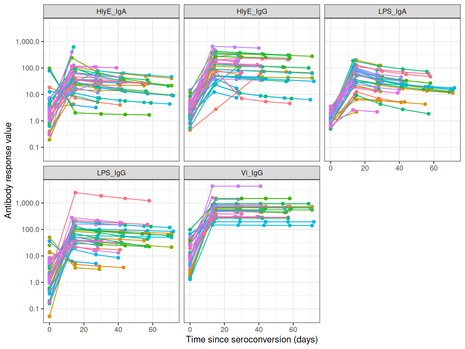

Running the Bayesian Model

The main function run_mod() fits a Bayesian MCMC model to estimate antibody dynamic curve parameters:

• y0: Baseline antibody concentration
• y1: Peak antibody concentration
  
• t1: Time to peak
• shape: Shape parameter
• alpha: Decay rate

# Note: This example uses reduced iterations for demonstration
# For actual analysis, use larger values (e.g., nmc=1000, niter=2000)

fitted_model <- run_mod(
  data = simulated_data,
  file_mod = serodynamics_example("model.jags"),
  nchain = 2,      # Number of MCMC chains
  nadapt = 100,    # Adaptation iterations
  nburn = 100,     # Burn-in iterations  
  nmc = 10,        # Samples per chain (use 1000+ for real analysis)
  niter = 20       # Total iterations (use 2000+ for real analysis)
)
#> Calling 2 simulations using the parallel method...
#> Following the progress of chain 1 (the program will wait for all chains
#> to finish before continuing):
#> Welcome to JAGS 4.3.2 on Thu Jan 22 06:29:44 2026
#> JAGS is free software and comes with ABSOLUTELY NO WARRANTY
#> Loading module: basemod: ok
#> Loading module: bugs: ok
#> . . Reading data file data.txt
#> . Compiling model graph
#>    Resolving undeclared variables
#>    Allocating nodes
#> Graph information:
#>    Observed stochastic nodes: 815
#>    Unobserved stochastic nodes: 285
#>    Total graph size: 14771
#> . Reading parameter file inits1.txt
#> . Initializing model
#> . Adapting 100
#> -------------------------------------------------| 100
#> ++++++++++++++++++++++++++++++++++++++++++++++++++ 100%
#> Adaptation incomplete.
#> . Updating 100
#> -------------------------------------------------| 100
#> ************************************************** 100%
#> . . . . . . Updating 20
#> . . . . Updating 0
#> . Deleting model
#> . 
#> All chains have finished
#> Warning: The adaptation phase of one or more models was not completed in 100
#> iterations, so the current samples may not be optimal - try increasing the
#> number of iterations to the "adapt" argument
#> Simulation complete.  Reading coda files...
#> Coda files loaded successfully
#> Finished running the simulation

head(fitted_model)
#> # A tibble: 6 × 7
#>   Iteration Chain Parameter Iso_type Stratification Subject  value
#>       <int> <int> <chr>     <chr>    <chr>          <chr>    <dbl>
#> 1         1     1 alpha     HlyE_IgA None           1       0.0114
#> 2         2     1 alpha     HlyE_IgA None           1       0.0114
#> 3         3     1 alpha     HlyE_IgA None           1       0.0114
#> 4         4     1 alpha     HlyE_IgA None           1       0.0114
#> 5         5     1 alpha     HlyE_IgA None           1       0.0217
#> 6         6     1 alpha     HlyE_IgA None           1       0.0217

Model Diagnostics

After fitting the model, check convergence diagnostics:

# Trace plots to assess chain mixing
plot_jags_trace(fitted_model)
#> $None
#> $None$HlyE_IgA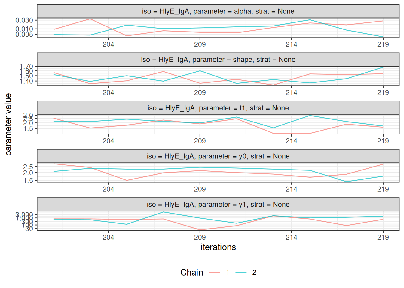

#>
#> $None$HlyE_IgG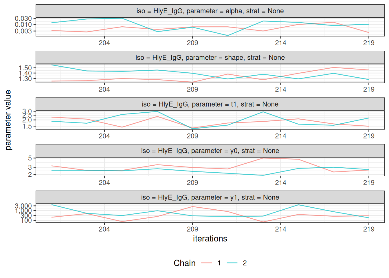

#>
#> $None$LPS_IgA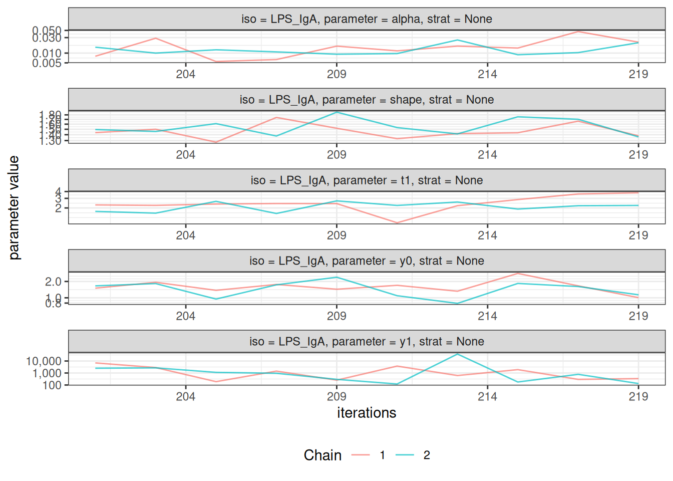

#>
#> $None$LPS_IgG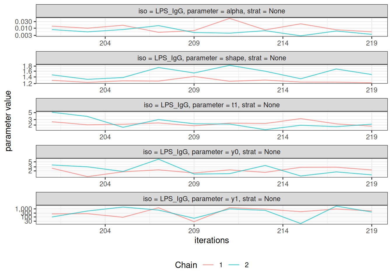

#>
#> $None$Vi_IgG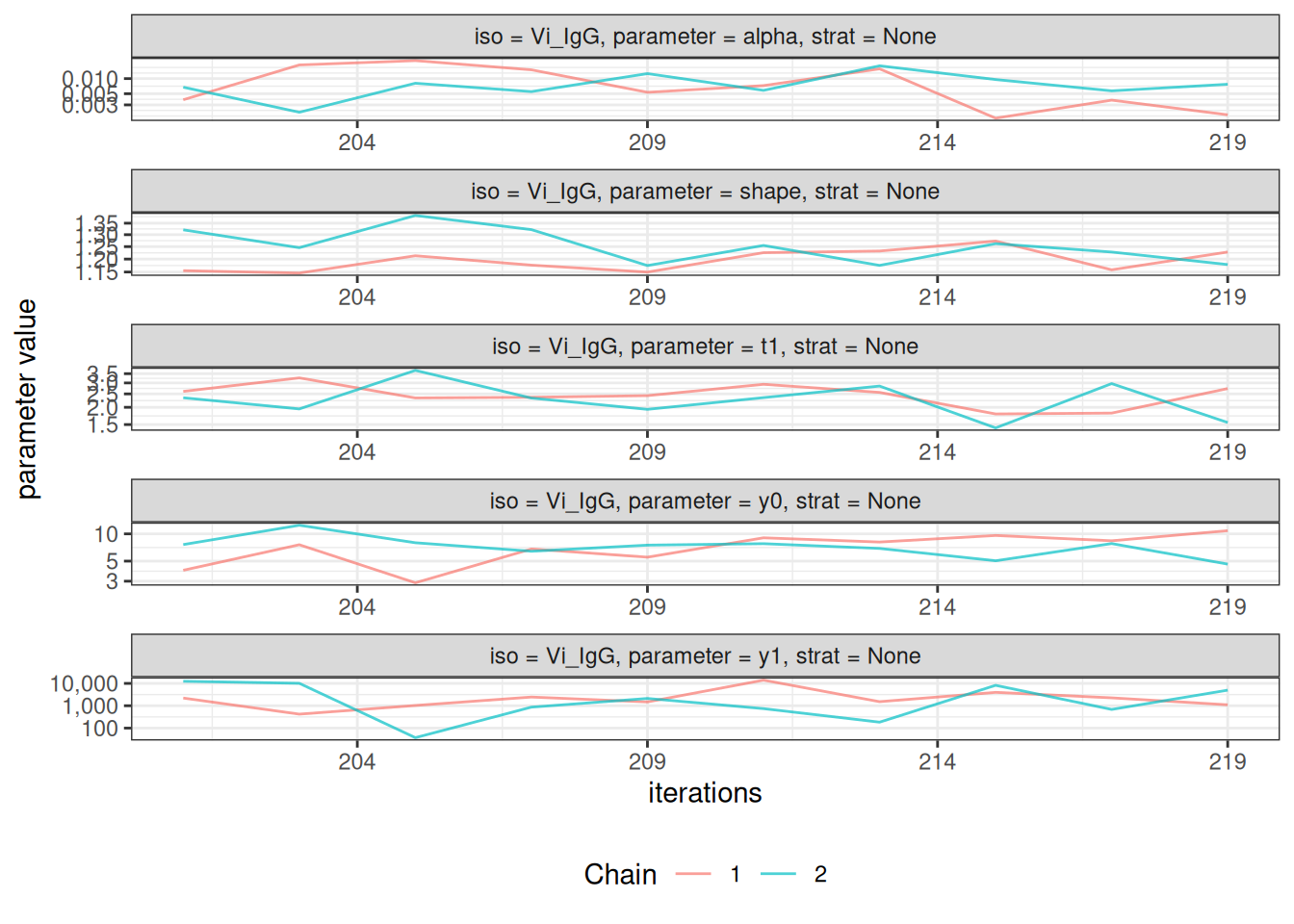

# Density plots of posterior distributions
plot_jags_dens(fitted_model)
#> $None
#> $None$HlyE_IgA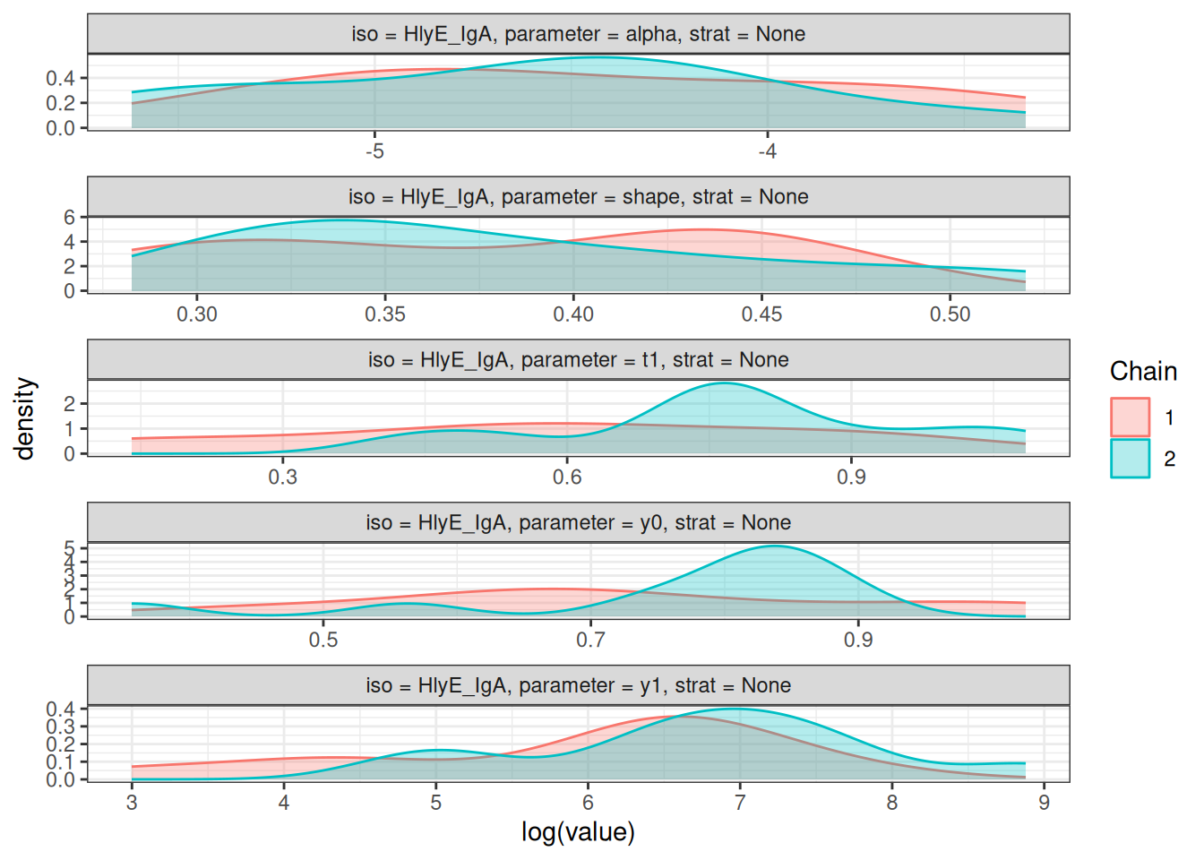

#>
#> $None$HlyE_IgG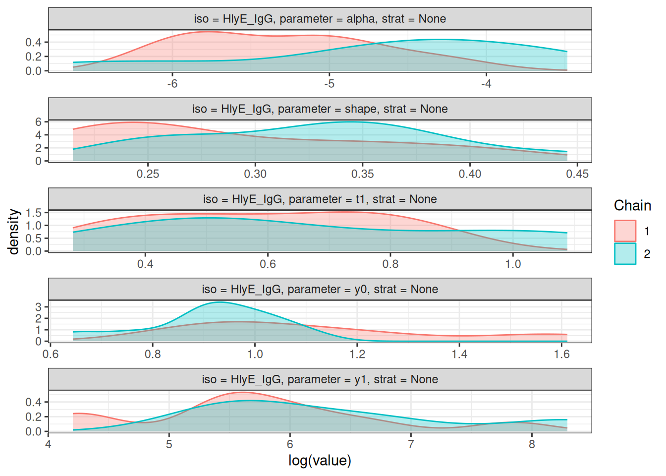

#>
#> $None$LPS_IgA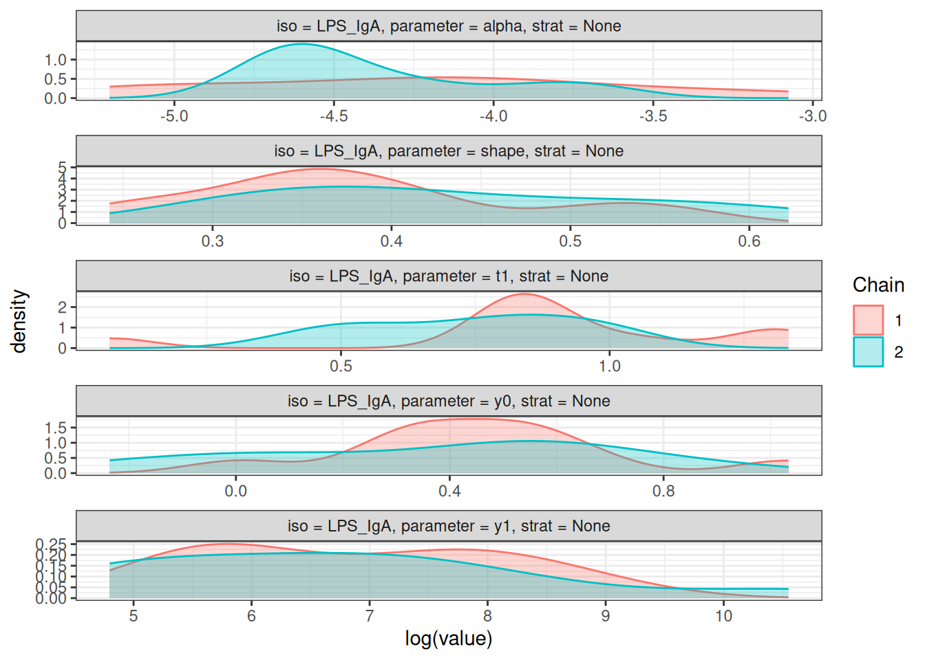

#>
#> $None$LPS_IgG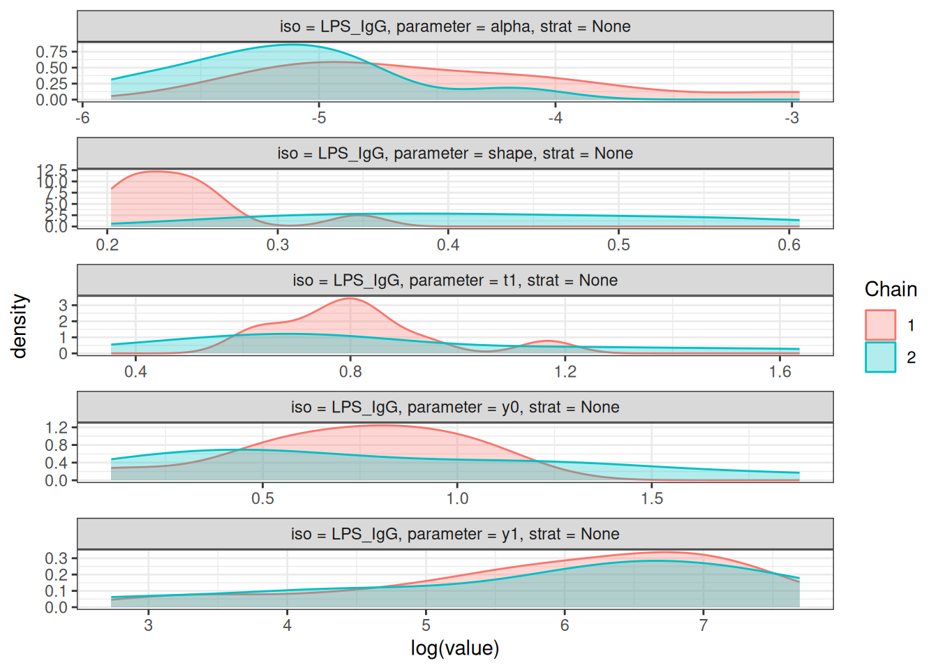

#>
#> $None$Vi_IgG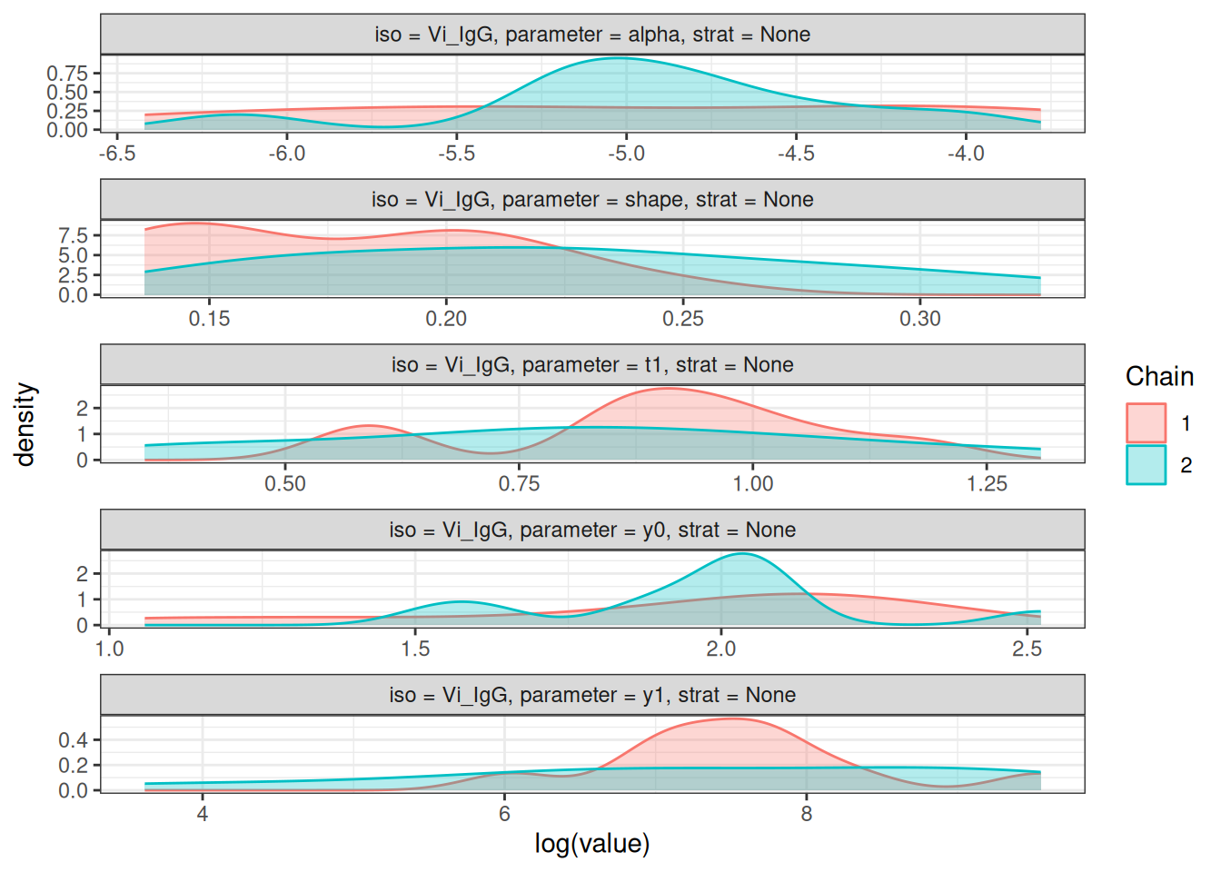

# Rhat statistics (values near 1.0 indicate convergence)
plot_jags_Rhat(fitted_model)
#> $None
#> $None$HlyE_IgA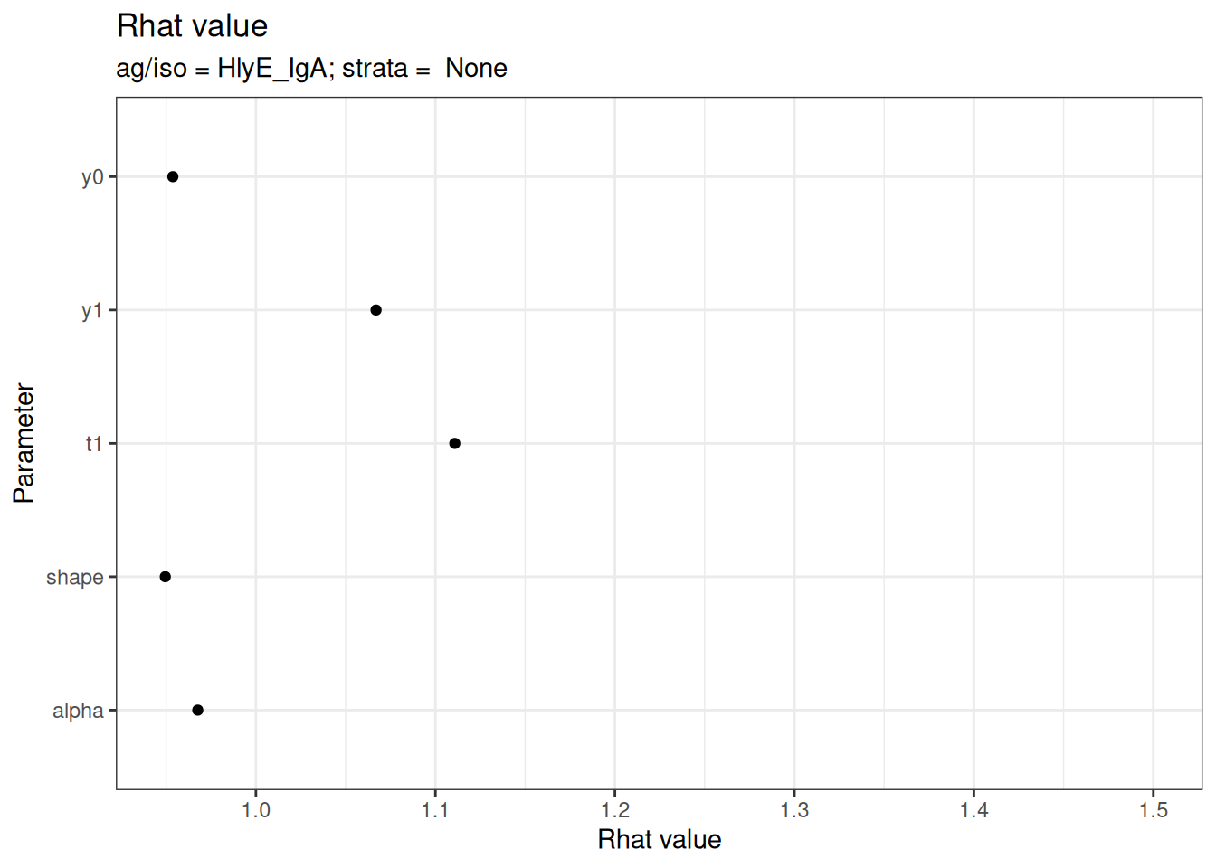

#>
#> $None$HlyE_IgG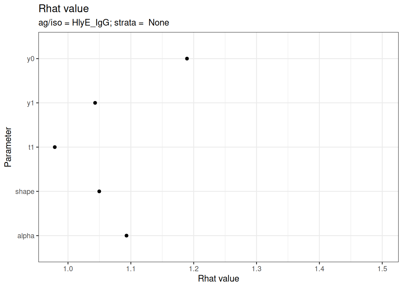

#>
#> $None$LPS_IgA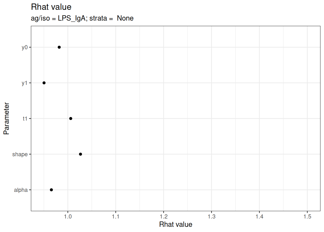

#>
#> $None$LPS_IgG

#>
#> $None$Vi_IgG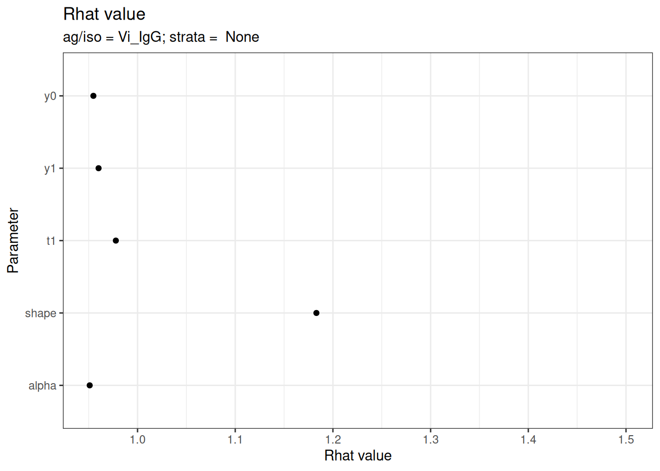

# Effective sample size
plot_jags_effect(fitted_model)
#> $None
#> $None$HlyE_IgA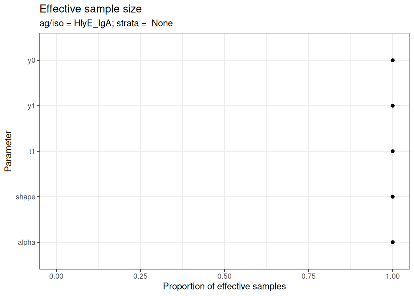

#>
#> $None$HlyE_IgG

#>
#> $None$LPS_IgA

#>
#> $None$LPS_IgG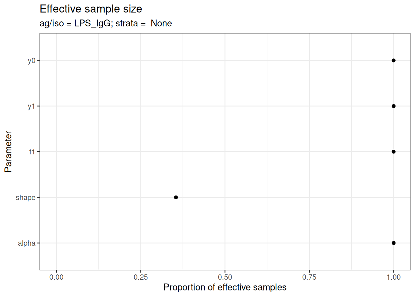

#>
#> $None$Vi_IgG

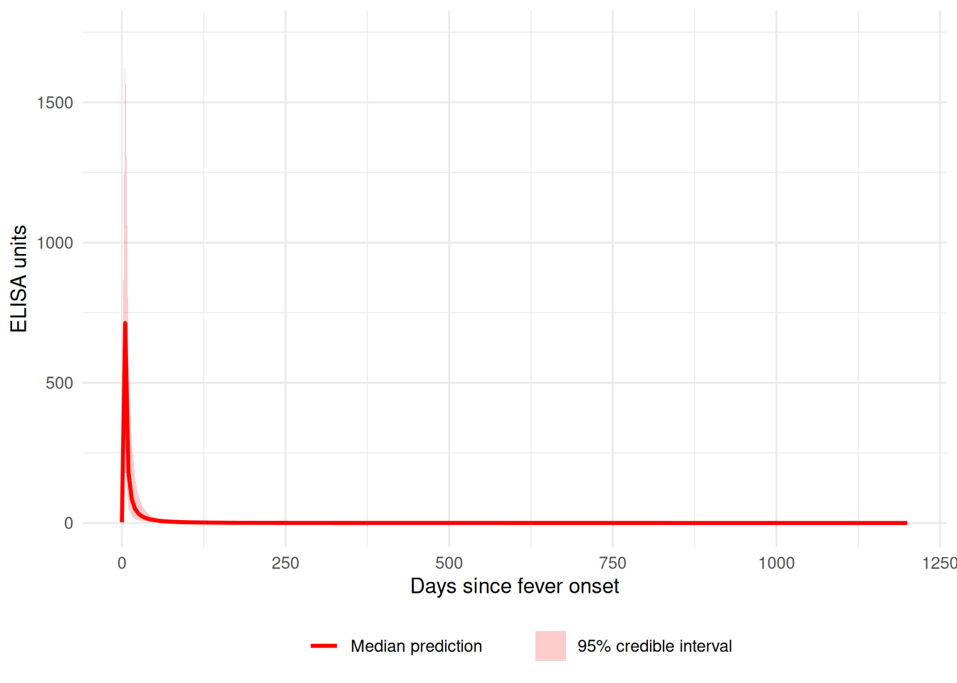
Visualizing Fitted Curves

Plot the predicted antibody curves with credible intervals:

plot_predicted_curve(
  fitted_model,
  ids = serocalculator::ids(simulated_data)[1],
  antigen_iso = simulated_data$antigen_iso[1]
)

Evaluating Individual-Level Fit Using Residual Metrics

After visualizing the model predictions, it’s important to quantify how well the posterior predictions match the observed data. The compute_residual_metrics() function provides objective measures of model fit at the individual level.

Computing Residual Metrics

Residual metrics complement visual assessments by providing quantitative summaries of prediction accuracy:

# Compute summary metrics for the first individual
first_id <- serocalculator::ids(simulated_data)[1]
first_antigen <- simulated_data$antigen_iso[1]

# Get summary metrics (MAE, RMSE, SSE)
residual_summary <- compute_residual_metrics(
  model = fitted_model,
  dataset = simulated_data,
  ids = first_id,
  antigen_iso = first_antigen,
  scale = "original",
  summary_level = "id_antigen"
)

print(residual_summary)
#> # A tibble: 1 × 6
#>   id    antigen_iso   MAE  RMSE   SSE n_obs
#>   <chr> <fct>       <dbl> <dbl> <dbl> <int>
#> 1 1     HlyE_IgA     22.1  30.6 2808.     3

The output shows:

• MAE (Mean Absolute Error): Average absolute difference between observed and predicted values
• RMSE (Root Mean Squared Error): Square root of average squared differences
• SSE (Sum of Squared Errors): Total squared prediction error
• n_obs: Number of observations used in the calculation

Examining Pointwise Residuals

For detailed diagnostics, you can examine residuals at each observed timepoint:

# Get pointwise residuals
pointwise <- compute_residual_metrics(
  model = fitted_model,
  dataset = simulated_data,
  ids = first_id,
  antigen_iso = first_antigen,
  scale = "original",
  summary_level = "pointwise"
)

print(pointwise)
#> # A tibble: 3 × 10
#>   id    antigen_iso     t    obs pred_med pred_lower pred_upper residual
#>   <chr> <fct>       <dbl>  <dbl>    <dbl>      <dbl>      <dbl>    <dbl>
#> 1 1     HlyE_IgA        0  0.666     2.41       1.78       2.67    -1.74
#> 2 1     HlyE_IgA       14 45.7      96.9       28.3      324.     -51.3 
#> 3 1     HlyE_IgA       27 43.1      29.9        8.37      84.5     13.2 
#> # ℹ 2 more variables: abs_residual <dbl>, sq_residual <dbl>

The pointwise output includes:

• obs: Observed antibody value
• pred_med: Posterior median prediction
• pred_lower / pred_upper: 95% credible interval
• residual: Raw residual (obs - pred)
• abs_residual: Absolute residual
• sq_residual: Squared residual

Comparing Multiple Individuals

You can compute metrics across multiple individuals to assess overall model performance:

# Get summary for multiple individuals
multi_id_summary <- compute_residual_metrics(
  model = fitted_model,
  dataset = simulated_data,
  ids = serocalculator::ids(simulated_data)[1:3],
  antigen_iso = first_antigen,
  scale = "original",
  summary_level = "id_antigen"
)

print(multi_id_summary)
#> # A tibble: 1 × 6
#>   id    antigen_iso   MAE  RMSE   SSE n_obs
#>   <chr> <fct>       <dbl> <dbl> <dbl> <int>
#> 1 1     HlyE_IgA     22.1  30.6 2808.     3

Log-Scale Residuals

For models fit on log-transformed data, compute residuals on the log scale:

# Compute log-scale residuals
log_residuals <- compute_residual_metrics(
  model = fitted_model,
  dataset = simulated_data,
  ids = first_id,
  antigen_iso = first_antigen,
  scale = "log",
  summary_level = "id_antigen"
)

print(log_residuals)
#> # A tibble: 1 × 6
#>   id    antigen_iso   MAE  RMSE   SSE n_obs
#>   <chr> <fct>       <dbl> <dbl> <dbl> <int>
#> 1 1     HlyE_IgA    0.801 0.885  2.35     3

Recommendation: Use residual metrics as a routine posterior predictive diagnostic step after fitting models with run_mod(). These metrics help identify individuals with poor fit and support objective model comparison.

Post-Processing Results

Extract and summarize the posterior estimates:

# Summarize parameter estimates
summary_stats <- post_summ(fitted_model)
print(summary_stats)
#> # A tibble: 25 × 11
#>    Iso_type Parameter Stratification       Mean       SD  Median  `2.5%` `25.0%`
#>    <chr>    <chr>     <chr>               <dbl>    <dbl>   <dbl>   <dbl>   <dbl>
#>  1 HlyE_IgA alpha     None              0.0132   9.15e-3 1.08e-2 3.87e-3 6.37e-3
#>  2 HlyE_IgA shape     None              1.47     1.01e-1 1.44e+0 1.34e+0 1.39e+0
#>  3 HlyE_IgA t1        None              2.02     4.93e-1 2.07e+0 1.15e+0 1.67e+0
#>  4 HlyE_IgA y0        None              2.13     3.68e-1 2.17e+0 1.46e+0 1.89e+0
#>  5 HlyE_IgA y1        None           1105.       1.55e+3 7.14e+2 4.82e+1 4.59e+2
#>  6 HlyE_IgG alpha     None              0.00956  8.14e-3 6.50e-3 1.77e-3 3.22e-3
#>  7 HlyE_IgG shape     None              1.36     9.20e-2 1.38e+0 1.25e+0 1.28e+0
#>  8 HlyE_IgG t1        None              1.94     4.89e-1 1.80e+0 1.35e+0 1.57e+0
#>  9 HlyE_IgG y0        None              2.85     7.70e-1 2.60e+0 2.01e+0 2.49e+0
#> 10 HlyE_IgG y1        None            833.       1.19e+3 2.95e+2 7.01e+1 2.42e+2
#> # ℹ 15 more rows
#> # ℹ 3 more variables: `50.0%` <dbl>, `75.0%` <dbl>, `97.5%` <dbl>

Working with Stratified Data

You can stratify the analysis by a grouping variable:

# Create stratified data
strat1 <- sim_case_data(
  n = 30, 
  curve_params = serocalculator::typhoid_curves_nostrat_100
) |>
  mutate(pathogen = "Typhoid")

strat2 <- sim_case_data(
  n = 30,
  curve_params = serocalculator::typhoid_curves_nostrat_100  
) |>
  mutate(pathogen = "Paratyphoid")

stratified_data <- bind_rows(strat1, strat2)

# Fit model with stratification
fitted_stratified <- run_mod(
  data = stratified_data,
  file_mod = serodynamics_example("model.jags"),
  nchain = 2,
  nadapt = 100,
  nburn = 100,
  nmc = 10,
  niter = 20,
  strat = "pathogen"  # Specify stratification variable
)
#> Calling 2 simulations using the parallel method...
#> Following the progress of chain 1 (the program will wait for all chains
#> to finish before continuing):
#> Welcome to JAGS 4.3.2 on Thu Jan 22 06:29:58 2026
#> JAGS is free software and comes with ABSOLUTELY NO WARRANTY
#> Loading module: basemod: ok
#> Loading module: bugs: ok
#> . . Reading data file data.txt
#> . Compiling model graph
#>    Resolving undeclared variables
#>    Allocating nodes
#> Graph information:
#>    Observed stochastic nodes: 775
#>    Unobserved stochastic nodes: 185
#>    Total graph size: 12303
#> . Reading parameter file inits1.txt
#> . Initializing model
#> . Adapting 100
#> -------------------------------------------------| 100
#> ++++++++++++++++++++++++++++++++++++++++++++++++++ 100%
#> Adaptation incomplete.
#> . Updating 100
#> -------------------------------------------------| 100
#> ************************************************** 100%
#> . . . . . . Updating 20
#> . . . . Updating 0
#> . Deleting model
#> . 
#> All chains have finished
#> Warning: The adaptation phase of one or more models was not completed in 100
#> iterations, so the current samples may not be optimal - try increasing the
#> number of iterations to the "adapt" argument
#> Simulation complete.  Reading coda files...
#> Coda files loaded successfully
#> Finished running the simulation
#> Calling 2 simulations using the parallel method...
#> Following the progress of chain 1 (the program will wait for all chains
#> to finish before continuing):
#> Welcome to JAGS 4.3.2 on Thu Jan 22 06:30:00 2026
#> JAGS is free software and comes with ABSOLUTELY NO WARRANTY
#> Loading module: basemod: ok
#> Loading module: bugs: ok
#> . . Reading data file data.txt
#> . Compiling model graph
#>    Resolving undeclared variables
#>    Allocating nodes
#> Graph information:
#>    Observed stochastic nodes: 760
#>    Unobserved stochastic nodes: 185
#>    Total graph size: 12135
#> . Reading parameter file inits1.txt
#> . Initializing model
#> . Adapting 100
#> -------------------------------------------------| 100
#> ++++++++++++++++++++++++++++++++++++++++++++++++++ 100%
#> Adaptation incomplete.
#> . Updating 100
#> -------------------------------------------------| 100
#> ************************************************** 100%
#> . . . . . . Updating 20
#> . . . . Updating 0
#> . Deleting model
#> . 
#> All chains have finished
#> Warning: The adaptation phase of one or more models was not completed in 100
#> iterations, so the current samples may not be optimal - try increasing the
#> number of iterations to the "adapt" argument
#> Simulation complete.  Reading coda files...
#> Coda files loaded successfully
#> Finished running the simulation

Next Steps

• See the function reference for complete API documentation
• Check out example datasets: ?nepal_sees, ?nepal_sees_jags_output

Session Info

sessioninfo::session_info()
#> ─ Session info ───────────────────────────────────────────────────────────────
#>  setting  value
#>  version  R version 4.5.2 (2025-10-31)
#>  os       Ubuntu 24.04.3 LTS
#>  system   x86_64, linux-gnu
#>  ui       X11
#>  language en-US
#>  collate  C.UTF-8
#>  ctype    C.UTF-8
#>  tz       UTC
#>  date     2026-01-22
#>  pandoc   3.1.11 @ /opt/hostedtoolcache/pandoc/3.1.11/x64/ (via rmarkdown)
#>  quarto   1.8.27 @ /usr/local/bin/quarto
#> 
#> ─ Packages ───────────────────────────────────────────────────────────────────
#>  package        * version    date (UTC) lib source
#>  cli              3.6.5      2025-04-23 [1] CRAN (R 4.5.2)
#>  coda             0.19-4.1   2024-01-31 [1] CRAN (R 4.5.2)
#>  codetools        0.2-20     2024-03-31 [3] CRAN (R 4.5.2)
#>  digest           0.6.39     2025-11-19 [1] CRAN (R 4.5.2)
#>  doParallel       1.0.17     2022-02-07 [1] CRAN (R 4.5.2)
#>  dplyr          * 1.1.4      2023-11-17 [1] CRAN (R 4.5.2)
#>  evaluate         1.0.5      2025-08-27 [1] CRAN (R 4.5.2)
#>  farver           2.1.2      2024-05-13 [1] CRAN (R 4.5.2)
#>  fastmap          1.2.0      2024-05-15 [1] CRAN (R 4.5.2)
#>  foreach          1.5.2      2022-02-02 [1] CRAN (R 4.5.2)
#>  fs               1.6.6      2025-04-12 [1] CRAN (R 4.5.2)
#>  generics         0.1.4      2025-05-09 [1] CRAN (R 4.5.2)
#>  GGally           2.4.0      2025-08-23 [1] CRAN (R 4.5.2)
#>  ggmcmc           1.5.1.2    2025-10-02 [1] CRAN (R 4.5.2)
#>  ggplot2        * 4.0.1      2025-11-14 [1] CRAN (R 4.5.2)
#>  ggstats          0.12.0     2025-12-22 [1] CRAN (R 4.5.2)
#>  glue             1.8.0      2024-09-30 [1] CRAN (R 4.5.2)
#>  gtable           0.3.6      2024-10-25 [1] CRAN (R 4.5.2)
#>  htmltools        0.5.9      2025-12-04 [1] CRAN (R 4.5.2)
#>  iterators        1.0.14     2022-02-05 [1] CRAN (R 4.5.2)
#>  jsonlite         2.0.0      2025-03-27 [1] CRAN (R 4.5.2)
#>  knitr            1.51       2025-12-20 [1] CRAN (R 4.5.2)
#>  labeling         0.4.3      2023-08-29 [1] CRAN (R 4.5.2)
#>  lattice          0.22-7     2025-04-02 [3] CRAN (R 4.5.2)
#>  lifecycle        1.0.5      2026-01-08 [1] CRAN (R 4.5.2)
#>  magrittr         2.0.4      2025-09-12 [1] CRAN (R 4.5.2)
#>  MASS             7.3-65     2025-02-28 [3] CRAN (R 4.5.2)
#>  otel             0.2.0      2025-08-29 [1] CRAN (R 4.5.2)
#>  pillar           1.11.1     2025-09-17 [1] CRAN (R 4.5.2)
#>  pkgconfig        2.0.3      2019-09-22 [1] CRAN (R 4.5.2)
#>  purrr            1.2.1      2026-01-09 [1] CRAN (R 4.5.2)
#>  R6               2.6.1      2025-02-15 [1] CRAN (R 4.5.2)
#>  RColorBrewer     1.1-3      2022-04-03 [1] CRAN (R 4.5.2)
#>  Rcpp             1.1.1      2026-01-10 [1] CRAN (R 4.5.2)
#>  rlang            1.1.7      2026-01-09 [1] CRAN (R 4.5.2)
#>  rmarkdown        2.30       2025-09-28 [1] CRAN (R 4.5.2)
#>  rngtools         1.5.2      2021-09-20 [1] CRAN (R 4.5.2)
#>  runjags        * 2.2.2-5    2025-04-09 [1] CRAN (R 4.5.2)
#>  S7               0.2.1      2025-11-14 [1] CRAN (R 4.5.2)
#>  scales           1.4.0      2025-04-24 [1] CRAN (R 4.5.2)
#>  serocalculator   1.4.0.9003 2026-01-22 [1] Github (ucd-serg/serocalculator@f340b9f)
#>  serodynamics   * 0.0.0.9048 2026-01-22 [1] local
#>  sessioninfo      1.2.3      2025-02-05 [1] any (@1.2.3)
#>  tibble           3.3.1      2026-01-11 [1] CRAN (R 4.5.2)
#>  tidyr            1.3.2      2025-12-19 [1] CRAN (R 4.5.2)
#>  tidyselect       1.2.1      2024-03-11 [1] CRAN (R 4.5.2)
#>  utf8             1.2.6      2025-06-08 [1] CRAN (R 4.5.2)
#>  vctrs            0.7.0      2026-01-16 [1] CRAN (R 4.5.2)
#>  withr            3.0.2      2024-10-28 [1] CRAN (R 4.5.2)
#>  xfun             0.56       2026-01-18 [1] CRAN (R 4.5.2)
#>  yaml             2.3.12     2025-12-10 [1] CRAN (R 4.5.2)
#> 
#>  [1] /home/runner/work/_temp/Library
#>  [2] /opt/R/4.5.2/lib/R/site-library
#>  [3] /opt/R/4.5.2/lib/R/library
#>  * ── Packages attached to the search path.
#> 
#> ──────────────────────────────────────────────────────────────────────────────